In cooperation with the California Solar & Storage Association, M.Cubed is releasing a white paper Rooftop Solar Reduces Costs for All Ratepayers.
As California policy makers seek to address energy affordability in 2025, this report shows why rooftop solar can and has helped control rate escalation. This research stands in direct contrast to claims that rooftop solar is to blame for rising rates. The report shows that the real reason electricity rates have increased dramatically in recent years is out-of-control utility spending and utility profit making, enabled by a lack of proper oversight by regulators.
This work builds on the original short report issued in November 2024, and subsequent replies to critiques by the Public Advocates Office and Professor Severin Borenstein. The supporting workpapers can be found here.
Policy makers wanting to address California’s affordability crisis should reject the utility’s so-called “solar cost shift” and instead partner with consumers who have helped save all ratepayers $1.5 billion in 2024 alone by investing in rooftop solar. The state should prioritize these resources that simultaneously reduce carbon, increase resiliency, and minimize grid spending. This realignment of energy priorities away from what works for investor-owned utilities – spending more on the grid – and toward what works for consumers – spending less – is particularly important in the face of increased electricity consumption due to electrification. More rooftop solar is needed, not less, to control costs for all ratepayers and meet the state’s clean energy goals.
Utilities have peddled a false “cost shift” theory that is based on the concept of “departing load.” Utilities claim that the majority of their costs are fixed. When a customer generates their own power from onsite solar panels, the utilities claim this forces all other ratepayers to pick up a larger share of their “fixed” costs. A close look at hard data behind this theory, however, shows a different picture.
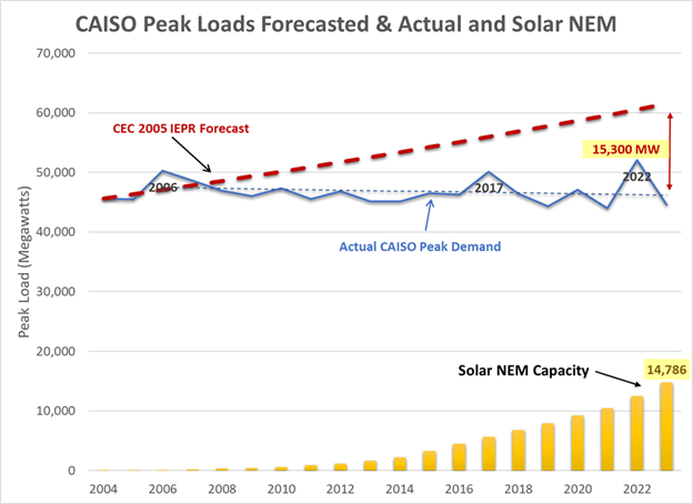
While California’s gross consumption – the “plug load” that is actual electricity consumption – has grown, that growth has been offset by customer-sited rooftop solar. This has kept the state’s peak consumption from the grid remarkably flat over the past twenty years, despite population growth, temperature increases, increased economic activity, and the rise in computers and other electronics in homes and businesses. Rooftop solar has not caused departing load in California. It has avoided load growth. By keeping our electric load on the grid flat, rooftop solar has avoided expensive grid expansion projects, in addition to reducing generation expenses, lowering costs for everyone.
Contrary to messaging from utilities and their regulators, California electricity consumption still peaks in mid-afternoon on hot summer days. There has been so much focus on the evening “net peak,” depicted by the “duck curve,” that many people have lost sight of the true peak. The annual peak in plug load happens when the sun is shining brightest. Clear, hot days lead to both high electricity usage from air conditioning and peak solar output.
The “net peak” is grid-based consumption minus generation from utility-scale solar and wind farms. It is an important dynamic to look at as we seek to reduce non-renewable sources of energy, and it shows us that energy storage will be essential going forward. However, an exclusive focus on net peak misses a bigger picture, particularly when looking at previously installed resources, and hides the value of solar energy.
California’s two million rooftop solar systems installed under net metering, including those that do not have batteries, continue to reduce statewide costs year after year by reducing the true peak. While most new solar systems now have batteries to address the evening net peak, historic solar continues to play a critical role in addressing the mid-day true peak.
Utilities and their regulators ignore these facts and focus the blame of rising rates on consumers seeking relief via rooftop solar. Politicians looking to address a growing crisis of energy affordability in California should reject the scapegoating of working- and middle-class families who have invested their own money in rooftop solar, and should instead promote the continued growth of this important distributed resource to meet growing needs for electricity.
The state is at a crossroads. As we power more of our cars, appliances, and heating with electricity, usage will increase dramatically. Relying entirely on utilities to deliver that energy from faraway power plants on long-distance power lines would involve massive delays and cause costs to rise even higher. Aggressive rooftop solar deployment could offset significant portions of the projected demand increase from electrification, helping control costs in the future.
The real reason for rate increases is runaway utility spending, driven by the utilities’ interest in increasing profits. Utility spending on grid infrastructure at the transmission and distribution levels has increased 130%-260% for each of the utilities over the past 8-12 years. These increases in spending track at a nearly 1:1 ratio with rate increases. This demonstrates that rates have gone up because utility spending has gone up. If utility costs were anything close to fixed and rates kept going up, there could be room for a cost shift argument. Or, if utility spending increased and rates increased significantly more, there could be a cost shift. The data shows neither of these trends. Rates have been increasing commensurate with spending, demonstrating that it is utility spending increases that have caused rates to increase, not consumers investing in clean energy.
Inspired by this faulty approach to measuring solar costs and benefits, the CPUC rolled out a transition from net metering to net billing that was abrupt and extreme. It has caused massive layoffs of skilled solar professionals and bankruptcies or closures of long-standing solar businesses. The poorly managed policy change set the market back ten years. A year and a half after the transition, the market still has not recovered.
California needs more rooftop solar and customer-sited batteries to contain costs and thereby rein in rate increases for all California ratepayers. To get the state back on track, policy makers need to stop attacking solar and adopt smart policies without delay.
• Respect the investments of customers who installed solar under NEM-1 and NEM-2. Do not change the terms of those contracts.
• Reject solar-specific taxes or fees in all forms, via the CPUC, the state budget, or local property taxes.
• Cut red tape in permitting and interconnection, and restore the right of solar contractors to install batteries. Do not use contractor licensing rules at the CSLB to restrict solar contractors from installing batteries.
• Establish a Million Solar Batteries initiative that includes virtual power plants and targeted incentives.
• Fix perverse utility profit motives that drive utilities to spend ratepayer money inefficiently, and even unnecessarily, and that motivate them to fight rooftop solar and other alternative ways to power California families and businesses.
• Launch a new investigation into utility oversight and overhaul the regulatory structure such that government regulators have the ability to properly scrutinize and contain utility spending.
California should be proud of its globally significant rooftop solar market. This solar development has diversified resources, served as a check on runaway utility spending, and helped clean the air all while tapping into private investments in clean energy. As the state looks to decarbonize its economy, the need to generate energy while minimizing capital intensive investments in grid infrastructure makes distributed solar and storage an even higher priority. State regulators need to stop being weak in utility oversight and exercise bold leadership for affordable clean energy that will benefit all ratepayers. California can start by getting back to promoting, not attacking, rooftop solar and batteries for all consumers.