Tag Archives: market price benchmark

How to properly calculate the marginal GHG emissions from electric vehicles and electrification

Recently the questions about whether electric vehicles increase greenhouse gas (GHG) emissions and tracking emissions directly to generation on a 24/7 basis have gained saliency. This focus on immediate grid-created emissions illustrates an important concept that is overlooked when looking at marginal emissions from electricity. The decision to consume electricity is more often created by a single large purchase or action, such as buying a refrigerator or a new electric vehicle, than by small decisions such as opening the refrigerator door or driving to the grocery store. Yet, the conventional analysis of marginal electricity costs and emissions assumes that we can arrive at a full accounting of those costs and emissions by summing up the momentary changes in electricity generation measured at the bulk power markets created by opening that door or driving to the store.

But that’s obviously misleading. The real consumption decision that created the marginal costs and emissions is when that item is purchased and connected to the grid. And on the other side, the comparative marginal decision is the addition of a new resource such as a power plant or an energy efficiency investment to serve that new increment of load.

So in that way, your flight to Boston is not whether you actually get on the plane, which is like opening the refrigerator door, but rather your purchase of the ticket which led to the incremental decision by the airline to add another scheduled flight. It’s the share of the fuel use for that added flight which is marginal, just as buying a refrigerator is responsible for the share of the energy from the generator added to serve the incremental long-term load.

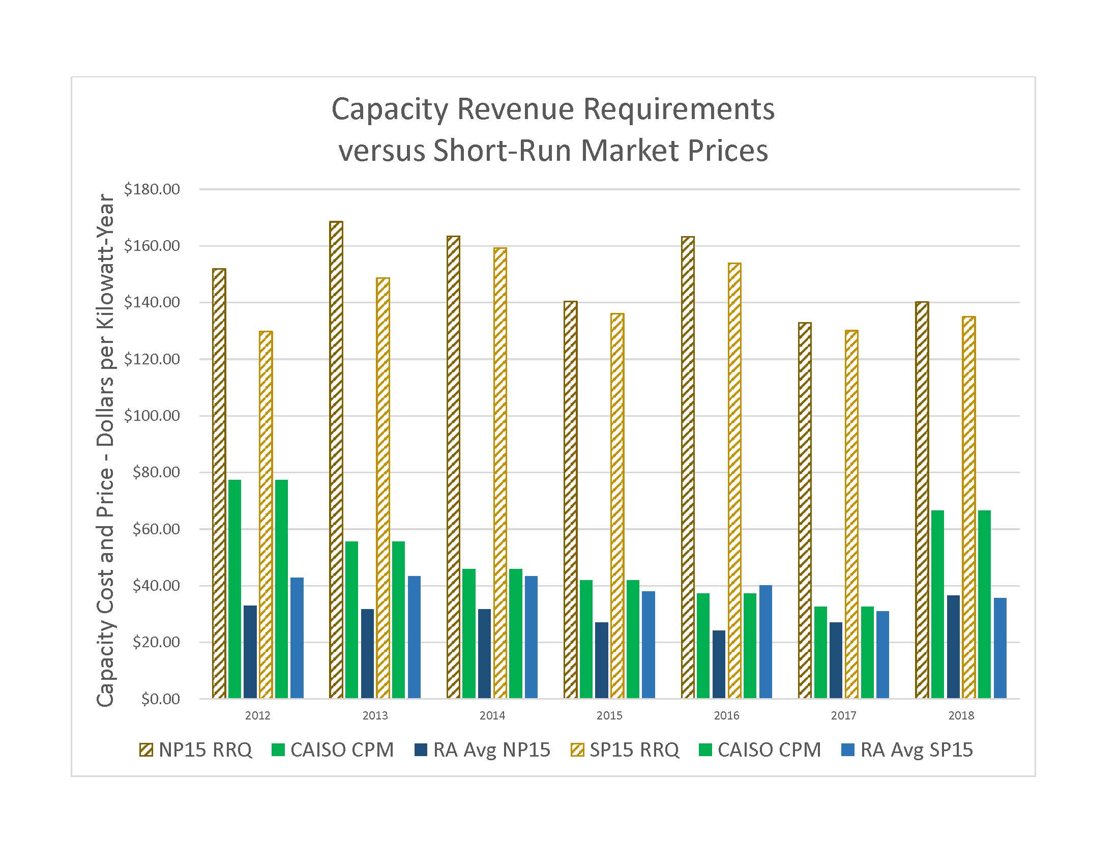
There are growing questions about the use of short run market prices as indicators of market value of generation assets for a number of reasons. This paper critiquing “surge” pricing on the grid has one set of aspects that undermine that principle.

Meredith Fowley at the Energy Institute at Haas compared two approaches to measuring the additional GHG emissions from a new electric vehicle. The NREL paper uses the correct approach of looking at longer term incremental resource additions rather than short run operating emissions. The hourly marginal energy use modeled by Holland et al (2022) is not particularly relevant to the question of GHG emissions from added load for several reasons and for that reason any study that doesn’t use a capacity expansion model will deliver erroneous results. In fact, you will get more accurate results from relying on a simple spreadsheet model using capacity expansion than a complex production cost hourly model.

In the electricity grid, added load generally doesn’t just require increased generation from existing plants, but rather it induces investment in new generation (or energy savings elsewhere, which have zero emissions) to meet capacity demands. This is where economists make a mistake thinking that the “marginal” unit is additional generation from existing plants–in a capacity limited system such as the electricity grid, its investment in new capacity.

That average emissions are falling as shown in Holland et al while hourly “marginal” emissions are rising illustrates this error in construction. Mathematically that cannot be happening if the marginal emission metric is correct. The problem is that Holland et al have misinterpreted the value they have calculated. It is in fact not the first derivative of the average emission function, but rather the second partial derivative. That measures the change in marginal emissions, not marginal emissions themselves. (And this is why long-run marginal costs are the relevant costing and pricing metric for electricity, not hourly prices.) Given that 75% of new generation assets in the U.S. were renewables, it’s difficult to see how “marginal” emissions are rising when the majority of new generation is GHG-free.

The second issue is that the “marginal” generation cannot be identified in ceteris paribus (i.e., all else held constant) isolation from all other policy choices. California has a high RPS and 100% clean generation target in the context of beneficial electrification of buildings and transportation. Without the latter, the former wouldn’t be pushed to those levels. The same thing is happening at the federal level. This means that the marginal emissions from building decarbonization and EVs are even lower than for more conventional emission changes.

Further, those consumers who choose beneficial electrification are much more likely to install distributed energy resources that are 100% emission free. Several studies show that 40% of EV owners install rooftop solar as well, far in excess of the state average, (In Australia its 60% of EV owners.) and they most likely install sufficient capacity to meet the full charging load of their EVs. So the system marginal emissions apply only to 60% of EV owners.

There may be a transition from hourly (or operational) to capacity expansion (or building) marginal or incremental emissions, but the transition should be fairly short so long as the system is operating near its reserve margin. (What to do about overbuilt systems is a different conversation.)

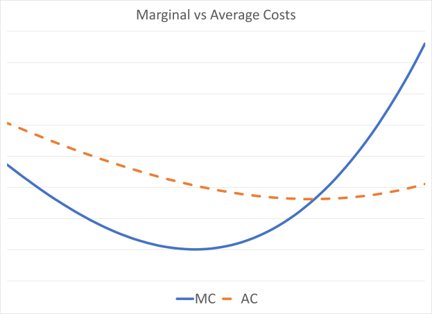
There’s deeper problem with the Holland et al papers. The chart that Fowlie pulls from the article showing that marginal emissions are rising above average emissions while average emissions are falling is not mathematically possible. (See for example, https://www.thoughtco.com/relationship-between-average-and-marginal-cost-1147863) For average emissions to be falling, marginal emissions must be falling and below average emissions. The hourly emissions are not “marginal” but more likely are the first derivative of the marginal emissions (i.e., the marginal emissions are falling at a decreasing rate.) If this relationship holds true for emissions, that also means that the same relationship holds for hourly market prices based on power plant hourly costs.

All of that said, it is important to incentivize charging during high renewable hours, but so long as we are adding renewables in a manner that quantitatively matches the added EV load, regardless of timing, we will still see falling average GHG emissions.

It is mathematically impossible for average emissions to fall while marginal emissions are rising if the marginal emission values are ABOVE the average emissions, as is the case in the Holland et al study. What analysts have heuristically called “marginal” emissions, i.e., hourly incremental fuel changes, are in fact, not “marginal”, but rather the first derivative of the marginal emissions. And as you point out the marginal change includes the addition of renewables as well as the change in conventional generation output. Marginal must include the entire mix of incremental resources. How marginal is measured, whether via change in output or over time doesn’t matter. The bottom line is that the term “marginal” must be used in a rigorous economic context, not in a casual manner as has become common.

Often the marginal costs do not fit the theoretical mathematical construct based on the first derivative in a calculus equation that economists point to. In many cases it is a very large discreet increment, and each consumer must be assigned a share of that large increment in a marginal cost analysis. The single most important fact is that for average costs to be rising, marginal costs must be above average costs. Right now in California, average costs for electricity are rising (rapidly) so marginal costs must be above those average costs. The only possible way of getting to those marginal costs is by going beyond just the hourly CAISO price to the incremental capital additions that consumption choices induce. It’s a crazy idea to claim that the first 99 consumers have a tiny marginal cost and then the 100th is assigned the responsibility for an entire new addition such as another flight scheduled or a new distribution upgrade.

We can consider the analogy to unit commitment, and even further to the continuous operation of nuclear power plants. The airline scheduled that flight in part based on the purchase of the plane ticket, not on the final decision just before the gate was closed. Not flying saved a miniscule amount of fuel, but the initial scheduling decision created the bulk of the fuel use for the flight. In a similar manner a power plant that is committed several days before an expected peak load burns fuels while idling in anticipation of that load. If that load doesn’t arrive, that plant avoids a small amount of fuel use, but focusing only on the hourly price or marginal fuel use ignores the fuel burned at a significant cost up to that point. Similarly, Diablo Canyon is run at a constant load year-round, yet there are significant periods–weeks and even months–where Diablo Canyon’s full operational costs are above the CAISO market clearing price average. The nuclear plant is run at full load constantly because it’s dispatch decision was made at the moment of interconnection, not each hour, or even each week or month, which would make economic sense. Renewables have a similar characteristic where they are “scheduled and dispatched” effectively at the time of interconnection. That’s when the marginal cost is incurred, not as “zero-cost” resources each hour.

Focusing solely on the small increment of fuel used as a true measure of “marginal” reflects a larger problem that is distorting economic analysis. No one looks at the marginal cost of petroleum production as the energy cost of pumping one more barrel from an existing well. It’s viewed as the cost of sinking another well in a high cost region, e.g., Kern County or the North Sea. The same needs to be true of air travel and of electricity generation. Adding one more unit isn’t just another inframarginal energy cost–it’s an implied aggregation of many incremental decisions that lead to addition of another unit of capacity. Too often economics is caught up in belief that its like classical physics and the rules of calculus prevail.

Part 2: A response to “Is Rooftop Solar Just Like Energy Efficiency?”

Severin Borenstein at the Energy Institute at Haas has written another blog post asserting that solar rooftop rates are inefficient and must changed radically. (I previously responded to an earlier post.) When looking at the efficiency of NEM rates, we need to look carefully at several elements of electricity market and the overall efficiency of utility ratemaking. We can see that we can come to a very different conclusion.

I filed testimony in the NEM 3.0 rulemaking last month where I calculated the incremental cost of transmission investment for new generation and the reduction in the CAISO peak load that looks to be attributable to solar rooftop.

  • Using FERC Form 1 and CEC powerplant data, I calculated that the incremental cost of transmission is $37/MWH. (And this is conservative due to a couple of assumptions I made.) Interestingly, I had done a similar calculation for AEP in the PJM interconnect and also came up with $37/MWH. This seems to be a robust value in the right neighborhood.
  • Load growth in California took a distinct change in trend in 2006 just as solar rooftop installations gained momentum. I found a 0.93 correlation between this change in trend and the amount of rooftop capacity installed. Using a simple trend, I calculated that the CAISO load decreased 6,000 MW with installation of 9,000 MW of rooftop solar. Looking at the 2005 CEC IEPR forecast, the peak reduction could be as large as 11,000 MW. CAISO also estimated in 2018 that rooftop solar displaced in $2.6 billion in transmission investment.

When we look at the utilities’ cost to acquire renewables and add in the cost of transmission, we see that the claim that grid-scale solar is so much cheaper than residential rooftop isn’t valid. The “green” market price benchmark used to set the PCIA shows that the average new RPS contract price in 2016 was still $92/MWH in 2016 and $74/MWH in 2017. These prices generally were for 30 year contracts, so the appropriate metric for comparing a NEM investment is against the vintage of RPS contracts signed in the year the rooftop project was installed. For 2016, adding in the transmission cost of $37/MWH, the comparable value is $129/MWH and in 2017, $111/MWH. In 2016, the average retail rates were $149/MWH for SCE, $183/MWH for PG&E and $205/MWH for SDG&E. (Note that PG&E’s rate had jumped $20/MWH in 2 years, while SCE’s had fallen $20/MWH.) In a “rough justice” way, the value of the displaced energy via rooftop solar was comparable to the retail rates which reflect the value of power to a customer, at least for NEM 1.0 and 2.0 customers. Rooftop solar was not “multiples” of grid scale solar.

These customers also took on investment risk. I calculated the payback period for a couple of customers around 2016 and found that a positive payback was dependent on utility rates rising at least 3% a year. This was not a foregone conclusion at the time because retail rates had actually be falling up to 2013 and new RPS contract prices were falling as well. No one was proposing to guarantee that these customers recover their investments if they made a mistake. That they are now instead benefiting is unwarranted hubris that ignores the flip side of the importance of investment risk–that investors who make a good efficient decision should reap the benefits. (We can discuss whether the magnitude of those benefits are fully warranted, but that’s a different one about distribution of income and wealth, not efficiency.)

Claiming that grid costs are fixed immutable amount simply isn’t a valid claim. SCE has been trying unsuccessfully to enact a “grid charge” with this claim since at least 2006. The intervening parties have successfully shown that grid costs in fact are responsive to reductions in demand. In addition, moving to a grid charge that creates a “ratchet effect” in revenue requirements where once a utility puts infrastructure in place, it faces no risk for poor investment decisions. On the other hand the utility can place its costs into ratebase and raise rates, which then raises the ratchet level on the fixed charge. One of the most important elements of a market economy that leads to efficient investment is that investors face the risk of not earning a return on an investment. That forces them to make prudent decisions. A “ratcheted” grid charge removes this risk even further for utilities. If we’re claiming that we are creating an “efficient” pricing policy, then we need to consider all sides of the equation.

The point that 50% of rooftop solar generation is used to offset internal use is important–while it may not be exactly like energy efficiency, it does have the most critical element of energy efficiency. That there are additional requirements to implement this is of second order importance, Otherwise we would think of demand response that uses dispatch controls as similarly distinct from EE. Those programs also require additional equipment and different rates. But in fact we sum those energy savings with LED bulbs and refrigerators.

An important element of the remaining 50% that is exported is that almost all of it is absorbed by neighboring houses and businesses on the same local circuit. Little of the power goes past the transformer at the top of the circuit. The primary voltage and transmission systems are largely unused. The excess capacity that remains on the system is now available for other customers to use. Whether investors should be able to recover their investment at the same annual rate in the face of excess capacity is an important question–in a competitive industry, the effective recovery rate would slow.

Finally, public purpose program (PPP) and wildfire mitigation costs are special cases that can be simply rolled up with other utility costs.

  • The majority of PPP charges are a form of a tax intended for income redistribution. That function is admirable, but it shows the standard problem of relying on a form of a sales tax to finance such programs. A sales tax discourages purchases which then reduces the revenues available for income transfers, which then forces an increase in the sales tax. It’s time to stop financing the CARE and FERA programs from utility rates.
  • Wildfire costs are created by a very specific subclass of customers who live in certain rural and wildlands-urban interface (WUI) areas. Those customers already received largely subsidized line extensions to install service and now we are unwilling to charge them the full cost of protecting their buildings. Once the state made the decision to socialize those costs instead, the costs became the responsibility of everyone, not just electricity customers. That means that these costs should be financed through taxes, not rates.

Again, if we are trying to make efficient policy, we need to look at the whole. It is is inefficient to finance these public costs through rates and it is incorrect to assert that there is an inefficient subsidy created if a set of customers are avoiding paying these rate components.

ERCOT has the peak period scarcity price too high

The freeze and resulting rolling outages in Texas in February highlighted the unique structure of the power market there. Customers and businesses were left with huge bills that have little to do with actual generation expenses. This is a consequence of the attempt by Texas to fit into an arcane interpretation of an economic principle where generators should be able to recover their investments from sales in just a few hours of the year. Problem is that basic of accounting for those cashflows does not match the true value of the power in those hours.

The Electric Reliability Council of Texas (ERCOT) runs an unusual wholesale electricity market that supposedly relies solely on hourly energy prices to provide the incentives for incenting new generation investment. However, ERCOT is using the same type of administratively-set subsidies to create enough potential revenue to cover investment costs. Further, a closer examination reveals that this price adder is set too high relative to actual consumer value for peak load power. All of this leads to a conclusion relying solely on short-run hourly prices as a proxy for the market value that accrues to new entrants is a misplaced metric.

The total ERCOT market first relies on side payments to cover commitment costs (which creates barriers to entry but that’s a separate issue) and second, it transfers consumer value through to the Operating Reserve Demand Curve (ORDC) that uses a fixed value of lost load (VOLL) in an arbitrary manner to create “opportunity costs” (more on that definition at a later time) so the market can have sufficient scarcity rents. This second price adder is at the core of ERCOT’s incentive system–energy prices alone are insufficient to support new generation investment. Yet ERCOT has ignored basic economics and set this value too high based on both available alternatives to consumers and basic regional budget constraints.

I started with an estimate of the number of hours where prices need the ORDC to be at full VOLL of $9000/MWH to recover the annual revenue requirements of combustion turbine (CT) investment based on the parameters we collected for the California Energy Commission. It turns out to be about 20 to 30 hours per year. Even if the cost in Texas is 30% less, this is still more 15 hours annually, every single year or on average. (That has not been happening in Texas to date.) Note for other independent system operators (ISO) such as the California ISO (CAISO), the price cap is $1,000 to $2,000/MWH.

I then calculated the cost of a customer instead using a home generator to meet load during those hours assuming a life of 10 to 20 years on the generator. That cost should set a cap on the VOLL to residential customers as the opportunity cost for them. The average unit is about $200/kW and an expensive one is about $500/kW. That cost ranges from $3 to $5 per kWh or $3,000 to $5,000/MWH. (If storage becomes more prevalent, this cost will drop significantly.) And that’s for customers who care about periodic outages–most just ride out a distribution system outage of a few hours with no backup. (Of course if I experienced 20 hours a year of outage, I would get a generator too.) This calculation ignores the added value of using the generator for other distribution system outages created by events like a hurricane hitting every few years, as happens in Texas. That drives down this cost even further, making the $9,000/MWH ORDC adder appear even more distorted.

The second calculation I did was to look at the cost of an extended outage. I used the outages during Hurricane Harvey in 2017 as a useful benchmark event. Based on ERCOT and U.S. Energy Information Reports reports, it looks like 1.67 million customers were without power for 4.5 days. Using the Texas gross state product (GSP) of $1.9 trillion as reported by the St. Louis Federal Reserve Bank, I calculated the economic value lost over 4.5 days, assuming a 100% loss, at $1.5 billion. If we assume that the electricity outage is 100% responsible for that loss, the lost economic value per MWH is just under $5,000/MWH. This represents the budget constraint on willingness to pay to avoid an outage. In other words, the Texas economy can’t afford to pay $9,000/MWH.

The recent set of rolling blackouts in Texas provides another opportunity to update this budget constraint calculation in a different circumstance. This can be done by determining the reduction in electricity sales and the decrease in state gross product in the period.

Using two independent methods, I come up with an upper bound of $5,000/MWH, and likely much less. One commentator pointed out that ERCOT would not be able achieve a sufficient planning reserve level at this price, but that statement is based on the premises that short-run hourly prices reflect full market values and will deliver the “optimal” resource mix. Neither is true.

This type of hourly pricing overemphasizes peak load reliability value and undervalues other attributes such as sustainability and resilience. These prices do not reflect the full incremental cost of adding new resources that deliver additional benefits during non-peak periods such as green energy, nor the true opportunity cost that is exercised when a generator is interconnected rather than during later operations. Texas has overbuilt its fossil-fueled generation thanks to this paradigm. It needs an external market based on long-run incremental costs to achieve the necessary environmental goals.

Exit fee market benchmarks threaten CCAs abilities to meet long term obligations

Capacity Net Revenue Adequacy 2001-2018CCAs may have to choose between complying with the long-term commitments specified in Senate Bill 350 and continuing to operate because they cannot acquire resources at the specified market price benchmarks that value the entire utility portfolio according to the CPUC.

The chart above compares the revenue shortfalls that need to be made up from other capacity sales products to finance resource additions. The CAISO has reported for every year since 2001 that its short-run market clearing prices that were adopted as the market price benchmark in the PCIA have been insufficient to support new conventional generation investment. The chart above shows the results of the CAISO Annual Report on Market Issues and Performance compiled from 2012 to 2018, separated by north (NP15 RRQ) and south (SP15 RRQ) revenue requirements for new resources. (The historic data shows that CAISO revenues have never been sufficient to finance a resource addition.) The CAISO signs capacity procurement (CPM) agreements to meet near-term reliability shortfalls which is one revenue source for a limited number of generators. The other short run price is the resource adequacy credits transacted by load serving entities (LSE) such as the utilities and CCAs. This revenue source is available to a broader set of resources. However, neither of revenues come close to closing the cost shortfall for new capacity.

The CPUC and the CAISO have deliberately suppressed these market prices to avoid the price spikes and reliability problems that occurred during the 2000-2001 energy crisis. By explicit state policy, these market prices are not to be used for assessing resource acquisition benchmarks. Yet, the CPUC adopted in its PCIA OIR decision (D.18-10-019) exactly this stance by asserting that the CCAs must be able to acquire new resources at less than these prices to beat the benchmarks used to calculate the PCIA. The CPUC used the CAISO energy prices plus the average RA prices as the base for the market value benchmark that represents the CCA threshold.

In a functioning market, the relevant market prices should indicate the relative supply-demand balance–if supply is short then prices should rise sufficiently to cover the cost of new entrants. Based on the relative price balance in the chart, no new capacity resources should be needed for some time.

Yet the CPUC recently issued a decision (D.19-04-040) that ordered procurement of 2,000 MW of capacity for resource adequacy. And now the CPUC proposes to up that target to 4,000 MW by 2021. All of this runs counter to the price signals that CPUC claims represent the “market value” of the assets held by the utilities.

If the CCAs purchase resources that cost more than the PCIA benchmarks then they will be losing money for their ratepayers (note that CCAs have no shareholders). Most often long-term power purchase agreements (PPA) have prices above the short-term prices because those short-term prices do not cover all of the values transacted in the market place. (More on that in the near future.) The CPUC should either align its market value benchmarks with its resource acquisition directives or acknowledge that their directives are incorrect.