Tag Archives: renewables

Discerning what drives rate increases is more complex than shown in LBNL study

The renewables policy team at Lawrence Berkeley National Laboratory (LBNL) released a study maintaining that it identifies the primary drivers of rate increases in the U.S. LBNL also issued a set of slides summarizing the study but there discrepancies between the two. (This post focuses on the study.)

First, this group of authors have been important leaders in tracking technology costs and resource alternatives at a micro level. You can find many of their studies cited in my various posts on renewables and distributed energy resources (DER). This time the authors may have stretched a bit too far.

Unfortunately this study is much more about correlation than causality. The authors hint at a more complex story that would require much more sophisticated regression analysis (e.g., two or three stage and fixed effects regressions) to untangle. Yet the report uses the term “driver” numerous places when “correlation” or “association” would be more appropriate.

Observations about Table 2 that displays the regression results and the discussion about findings in Section 4:

  • 4.2 Price trends varied by state: Prices rose in states that are internalizing environmental and other costs while states with falling rates were continuing to impose environmental hazards and other costs on their citizens as a subsidy to utility shareholders.
  • 4.4 Finding that rising growth decreases rates (load delta): This finding confuses a shift in customer composition with overall causality. The study found it was rising commercial loads, not overall loads, that decreased rates. That means the share of lower cost commercial customers increased, so, of course, the average rate decreased. The residential rates were unchanged statistically.
  • 4.5 Behind the meter (BTM) solar: the most egregious error. The authors acknowledge this issue is problematic with many different viewpoints, but then plow ahead anyway. Customers find the most effective way to respond to rising rates is to install their own generation. This is classic economic cause and effect, yet the authors run a model assuming the reverse.

The problem is that they accept as given the utility narrative that rooftop customers are shirking cost responsibility while ignore the cost saving from serving load themselves. The authors also buy into the false narrative that utilities have substantial “fixed” costs—every other industry that has large fixed costs recover those through variable charges.  That the BTM variable is strongly negative for the 2017-22 period and then positive for 2019-24 is an analytic red flag. (The negative value for the RPS effect from 2016-2021 just as California’s most expensive renewables came on line compared to the other periods is another red flag in the regression analysis overall.)

Our analysis shows instead how California NEM customers have saved money for other customers. The authors do not include that critique of the studies done in California in their citations. We also deeply critiqued the E3 study of Washington’s NEM program, finding numerous analytic and conceptual errors. (Ahmad Faruqui would disavow his Sergici et al 2019 study included as a supporting citation in the LBNL study.)

There are two fundamental conceptual errors in these underlying analyses that the LBNL authors rely on: 1) that utilities have the right to serve 100% of customer loads and customers must pay for the privilege to self serve with their own generation, and 2) that utilities are entitled to full recovery of all of their costs even when sales decrease. Neither of these premises hold in any other industry (even natural gas and water utilities).

Notably they found no statistical effect from energy efficiency programs yet the impacts on utility sales and revenues are identical to BTM solar. No one is calling for customers who install LED lighting, insulation or more efficient appliances to increase their contribution utility revenue requirements to be “fair.” The one difference is that DERs present the opportunity to truly “cut the cord” with the utility if rates become excessive. This is further evidence that this finding that rooftop solar unduly raises the rates for other customers is false and misleading.

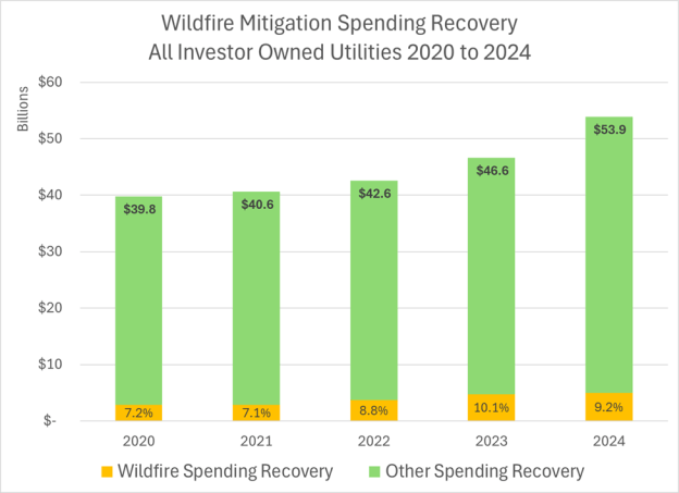
  • 4.9 Wildfire spending as a source of cost increases: the authors attribute a 6 cents/kWh increase in California wildfire spending. That’s incorrect (the PAO took PG&E’s assertion without checking it) as we have tracked the total utility spending—it’s only about 10% or less than 4 cents/kWh of IOU rates. But a portion of that increase already happened prior to 2019, and the wildfire bond adder wasn’t an increase but rather a repurposing of an existing bond cost recovery charge. The rate increase attributable to wildfire spending is less than 3 cents on a statewide basis (rolling in the municipals, e.g., LADWP & SMUD).

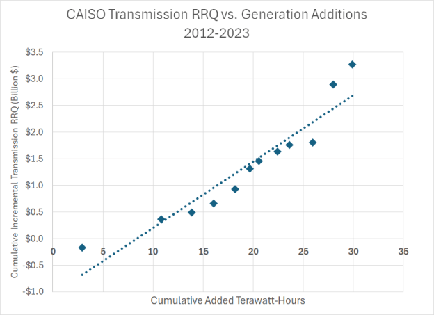
The real reason for California rate increases are: 1) unusual exposure to natural gas prices because the IOUs have not hedged power purchases 2) increase in resource adequacy prices because of multiple changes in how this handled (the underlying reason being to squeeze CCAs), 3) unregulated spending in distribution infrastructure the IOUs starting in 2010 and 3) a 150% increase in transmission investment to deliver grid scale renewable generation since 2012. 

CAISO Transmission Costly for New Generation

The California utilities have added substantial new generation over the last two decades while peak demand and energy loads have remained fairly constant. Based on Energy Information Administration data for 2012 to 2023 in the California Independent System Operator (CAISO) area, 75.7% of the generation added other than plant repowering is for renewables meeting the state’s Renewable Portfolio Standard.[1] Most of these new plants are located remotely from the majority of customer loads so transmission lines must be built to deliver that energy.

Over the same period from 2012 to 2023, the total annual transmission revenue requirements for the three investor-owned utilities (IOU) in the CAISO (i.e., PG&E, SCE and SDG&E), rose from $2.217 billion to $5.487 billion or 147%.[2] That is 7.8% per year.  The chart below compares the increase in transmission revenue and the addition of generation over that period.

Transmission spending is driven largely by additions of generation. This fact is particularly evident when transmission costs rise so rapidly despite no significant load growth. For this reason, the marginal or incremental cost should be expressed in dollars per kilowatt or kilowatt-hour. And because 76% of the new generation is for renewable energy, not for peak reliability, kilowatt-hours of energy is the best metric.

Using these two data sources, we updated the incremental or marginal cost for transmission using the change in annual revenue requirements as a proxy for the direct cost. The chart at the top shows how transmission revenue requirement increases relate to generation additions. Based on this analysis, the marginal cost of transmission is $125 per megawatt-hour or $0.1246 per kilowatt-hour.[3] Given that retail transmission rates for the three IOUs have on average increased 250% to $0.04016 per kilowatt-hour, this result is consistent with the economic principle that marginal costs are above average costs when average costs are rising.


[1] EIA 923, https://www.eia.gov/electricity/data/eia923/, and EIA 861, https://www.eia.gov/electricity/data/eia861/

[2] CPUC, AB 67 Reports to the Legislature.

[3] The R-squared is 0.881, and the standard error is $0.0138 per kilowatt-hour.

White paper on how rooftop solar is really a benefit to all ratepayers

In cooperation with the California Solar & Storage Association, M.Cubed is releasing a white paper Rooftop Solar Reduces Costs for All Ratepayers.

As California policy makers seek to address energy affordability in 2025, this report shows why rooftop solar can and has helped control rate escalation. This research stands in direct contrast to claims that rooftop solar is to blame for rising rates. The report shows that the real reason electricity rates have increased dramatically in recent years is out-of-control utility spending and utility profit making, enabled by a lack of proper oversight by regulators.

This work builds on the original short report issued in November 2024, and subsequent replies to critiques by the Public Advocates Office and Professor Severin Borenstein. The supporting workpapers can be found here.

Policy makers wanting to address California’s affordability crisis should reject the utility’s so-called “solar cost shift” and instead partner with consumers who have helped save all ratepayers $1.5 billion in 2024 alone by investing in rooftop solar. The state should prioritize these resources that simultaneously reduce carbon, increase resiliency, and minimize grid spending. This realignment of energy priorities away from what works for investor-owned utilities – spending more on the grid – and toward what works for consumers – spending less – is particularly important in the face of increased electricity consumption due to electrification. More rooftop solar is needed, not less, to control costs for all ratepayers and meet the state’s clean energy goals.

Utilities have peddled a false “cost shift” theory that is based on the concept of “departing load.” Utilities claim that the majority of their costs are fixed. When a customer generates their own power from onsite solar panels, the utilities claim this forces all other ratepayers to pick up a larger share of their “fixed” costs. A close look at hard data behind this theory, however, shows a different picture.

While California’s gross consumption – the “plug load” that is actual electricity consumption – has grown, that growth has been offset by customer-sited rooftop solar. This has kept the state’s peak consumption from the grid remarkably flat over the past twenty years, despite population growth, temperature increases, increased economic activity, and the rise in computers and other electronics in homes and businesses. Rooftop solar has not caused departing load in California. It has avoided load growth. By keeping our electric load on the grid flat, rooftop solar has avoided expensive grid expansion projects, in addition to reducing generation expenses, lowering costs for everyone.

Contrary to messaging from utilities and their regulators, California electricity consumption still peaks in mid-afternoon on hot summer days. There has been so much focus on the evening “net peak,” depicted by the “duck curve,” that many people have lost sight of the true peak. The annual peak in plug load happens when the sun is shining brightest. Clear, hot days lead to both high electricity usage from air conditioning and peak solar output.

The “net peak” is grid-based consumption minus generation from utility-scale solar and wind farms. It is an important dynamic to look at as we seek to reduce non-renewable sources of energy, and it shows us that energy storage will be essential going forward. However, an exclusive focus on net peak misses a bigger picture, particularly when looking at previously installed resources, and hides the value of solar energy.
California’s two million rooftop solar systems installed under net metering, including those that do not have batteries, continue to reduce statewide costs year after year by reducing the true peak. While most new solar systems now have batteries to address the evening net peak, historic solar continues to play a critical role in addressing the mid-day true peak.

Utilities and their regulators ignore these facts and focus the blame of rising rates on consumers seeking relief via rooftop solar. Politicians looking to address a growing crisis of energy affordability in California should reject the scapegoating of working- and middle-class families who have invested their own money in rooftop solar, and should instead promote the continued growth of this important distributed resource to meet growing needs for electricity.

The state is at a crossroads. As we power more of our cars, appliances, and heating with electricity, usage will increase dramatically. Relying entirely on utilities to deliver that energy from faraway power plants on long-distance power lines would involve massive delays and cause costs to rise even higher. Aggressive rooftop solar deployment could offset significant portions of the projected demand increase from electrification, helping control costs in the future.

The real reason for rate increases is runaway utility spending, driven by the utilities’ interest in increasing profits. Utility spending on grid infrastructure at the transmission and distribution levels has increased 130%-260% for each of the utilities over the past 8-12 years. These increases in spending track at a nearly 1:1 ratio with rate increases. This demonstrates that rates have gone up because utility spending has gone up. If utility costs were anything close to fixed and rates kept going up, there could be room for a cost shift argument. Or, if utility spending increased and rates increased significantly more, there could be a cost shift. The data shows neither of these trends. Rates have been increasing commensurate with spending, demonstrating that it is utility spending increases that have caused rates to increase, not consumers investing in clean energy.

Inspired by this faulty approach to measuring solar costs and benefits, the CPUC rolled out a transition from net metering to net billing that was abrupt and extreme. It has caused massive layoffs of skilled solar professionals and bankruptcies or closures of long-standing solar businesses. The poorly managed policy change set the market back ten years. A year and a half after the transition, the market still has not recovered.
California needs more rooftop solar and customer-sited batteries to contain costs and thereby rein in rate increases for all California ratepayers. To get the state back on track, policy makers need to stop attacking solar and adopt smart policies without delay.

• Respect the investments of customers who installed solar under NEM-1 and NEM-2. Do not change the terms of those contracts.
• Reject solar-specific taxes or fees in all forms, via the CPUC, the state budget, or local property taxes.
• Cut red tape in permitting and interconnection, and restore the right of solar contractors to install batteries. Do not use contractor licensing rules at the CSLB to restrict solar contractors from installing batteries.
• Establish a Million Solar Batteries initiative that includes virtual power plants and targeted incentives.
• Fix perverse utility profit motives that drive utilities to spend ratepayer money inefficiently, and even unnecessarily, and that motivate them to fight rooftop solar and other alternative ways to power California families and businesses.
• Launch a new investigation into utility oversight and overhaul the regulatory structure such that government regulators have the ability to properly scrutinize and contain utility spending.

California should be proud of its globally significant rooftop solar market. This solar development has diversified resources, served as a check on runaway utility spending, and helped clean the air all while tapping into private investments in clean energy. As the state looks to decarbonize its economy, the need to generate energy while minimizing capital intensive investments in grid infrastructure makes distributed solar and storage an even higher priority. State regulators need to stop being weak in utility oversight and exercise bold leadership for affordable clean energy that will benefit all ratepayers. California can start by getting back to promoting, not attacking, rooftop solar and batteries for all consumers.

California’s perceived “solar glut” problem is actually a “nuclear glut” problem

Several news stories have asserted that California has a “glut” of solar power that is being wasted and sold at a loss to other states. The problem is that the stories mischaracterize the situation, both in cause and magnitude.

The Diablo Canyon nuclear power units were scheduled to be retired in 2024 and 2025 due to having reached the end of their license and concerns around public safety from the aging plant. As a result, state energy regulators launched an aggressive renewable energy and battery storage procurement process in 2018 following the decision to close Diablo Canyon. Those added resources are now coming online to offset the anticipated loss of energy output from Diablo Canyon’s closure.

However, despite those additional renewable resources, the state legislature and Governor Newsom then extended the life of Diablo Canyon in 2022 to 2030. Diablo Canyon’s 2,200 megawatts of around-the-clock energy production – which adds up to 18 million megawatt hours a year – is the true source of grid management issues, particularly during the spring when the majority of energy curtailments occur.

This imbalance is exacerbated by the large swings in the state’s hydropower production, from 17 million megawatt hours during a dry 2022 to 30 million megawatt hours in a wet 2023. These swings are inherent in California’s power system, and related curtailments were common for decades before solar was on the scene. In other words, California will always need to have excess energy in wet years if it wants sufficient power in the other two-thirds of the years that are average or dry. Diablo Canyon’s year-round, around the clock output only makes that glut worse.

Not only is Diablo Canyon’s extension clogging up transmission lines and driving curtailment, it is also a high cost energy resource. PG&E initially claimed the Diablo Canyon power would cost about 5.5 cent per kilowatt hour, which is near the average cost of the California Independent System Operator’s (CAISO) energy purchases. Instead, PG&E is asking the California Public Utilities Commission to charge more than 9 cents per kilowatt hour, nearly double the cost of the average energy purchase.

Instead of blaming and halting California’s clean energy progress, an easier solution that would solve most of the curtailment issue would be to shut down Diablo Canyon from March to May, when energy demand is lowest in the state. This is when loads are lowest and hydro output the highest. Reducing at least some of Diablo Canyon’s 18 million megawatt hours per year, would more than offset the 3.2 million megawatt hours of solar energy that were curtailed in 2024. Diablo Canyon would still be available to meet summertime peaks. That would save ratepayers money and reduce the need to sell excess generation at a loss. 

California is already addressing other causes of curtailments by installing more storage capacity. It would be foolish to reduce solar generation now when we will need it in the near future to match the additional storage capacity. 

How California’s Rooftop Solar Customers Benefit Other Ratepayers Financially to the Tune of $1.5 Billion

The California Public Utilities Commission’s (CPUC) Public Advocates Office (PAO) issued in August 2024 an analysis that purported to show current rooftop solar customers are causing a “cost shift” onto non-solar customers amounting to $8.5 billion in 2024. Unfortunately, this rather simplistic analysis started from an incorrect base and left out significant contributions, many of which are unique to rooftop solar, made to the utilities’ systems and benefitting all ratepayers. After incorporating this more accurate accounting of benefits, the data (presented in the chart above) shows that rooftop solar customers will in fact save other ratepayers approximately $1.5 billion in 2024.

The following steps were made to adjust the original analysis presented by the PAO:

  1. Rates & Solar Output: The PAO miscalculates rates and overestimates solar output. Retail rates were calculated based on utilities’ advice letters and proceeding workpapers. They incorporate time-of-use rates according to the hours when an average solar customer is actually using and exporting electricity.  The averages are adjusted to include the share of net energy metering (NEM 1.0 and 2.0) and net billing tariff (NBT or “NEM 3.0”) customers (8% to 18% depending on the utility) who are receiving the California Alternate Rates for Energy program’s (CARE) low-income rate discount. (PAO assumed that all customers were non-CARE). In addition, the average solar panel capacity factor was reduced to 17.5% based on the state’s distributed solar database.[1] Accurately accounting for rates and solar outputs amounts to a $2.457 billion in benefits ignored by the PAO analysis.
  2. Self Generation: The PAO analysis included solar self-consumption as being obligated to pay full retail rates. Customers are not obligated to pay for energy to the utility for self generation. Solar output that is self-consumed by the solar customer was removed from the calculation. Inappropriately including self consumption as “lost” revenue in PAO analysis amounts to $3.989 billion in a phantom cost shift that should be set aside.
  3. Historic Utility Savings: The PAO fails to account for the full and accurate amount of savings and the shift in the system created by rooftop solar that has lowered costs and rates. The historic savings are based on distributed solar displacing 15,000 megawatts of peak load and 23,000 gigawatt-hours of energy since 2006 compared to the California Energy Commission’s (CEC) 2005 Integrated Energy Policy Report forecast.[2] Deferred generation capacity valuation starts with the CEC’s cost of a combustion turbine[3] and is trended to the marginal costs filed in the most recent decided general rate cases. Generation energy is the mix of average California Independent System Operator (CAISO) market prices in 2023,[4] and utilities’ average renewable energy contract prices.[5] Avoided transmission costs are conservatively set at the current unbundled retail transmission rate components. Distribution investment savings are the weighted average of the marginal costs included in the utilities’ general case filings from 2007 to 2021. Accounting for utility savings from distributed solar amounts to $2.165 billion ignored by the PAO’s calculation.
  4. Displaced CARE Subsidy: The PAO analysis does not account for savings from solar customers who would otherwise receive CARE subsidies. When CARE customers buy less energy from the utilities, it reduces the total cost of the CARE subsidy born by other ratepayers. This is equally true for energy efficiency. The savings to all non-CARE customers from displacing electricity consumption by CARE customers with self generation is calculated from the rate discount times that self generation. Accounting for reduced CARE subsidies amounts to $157 million in benefits ignored by the PAO analysis.
  5. Customer Bill Payments: The PAO analysis does not account for payments towards fixed costs made by solar customers. Most NEM customers do not offset all of their electricity usage with solar.[6] NEM customers pay an average of $80 to $160 per month, depending on the utility, after installing solar.[7] Their monthly bill payments more than cover what are purported fixed costs, such as the service transformer. A justification for the $24 per month customer charge was a purported under collection from rooftop solar customers.[8] Subtracting the variable costs represented by the Avoided Cost Calculator from these monthly payments, the remainder is the contribution to utility fixed costs, amounting to an average of $70 per month. (In comparison for example, PG&E proposed an average fixed charge of $51 per month in the income graduated fixed charge proceeding.[9]) There is no data available on average NBT bills, but NBT customers also pay at least $15 per month in a minimum fixed charge today.[10] Accounting for fixed cost payments adds $1.18 billion in benefits ignored by the PAO analysis.

The correct analytic steps are as follows:

NEM Net Benefits = [(kWh Generation [Corrected] – kWh Self Use) x Average Retail Rate Compensation [Corrected] )]
– [(kWh Generation [Corrected] – kWh Self Use) x Historic Utility Savings ($/kWh)]
– [CARE/FERA kWh Self Use x CARE/FERA Rate Discount ($/kWh)]
– [(kWh Delivered x (Average Retail Rate ($/kWh) – Historic Utility Savings $(kWh))]

NBT Net Benefits = [(kWh Generation [Corrected] – kWh Self Use) x Average Retail Rate Compensation [Corrected])]
– [(kWh Generation [Corrected] – kWh Self Use) x Avoided Cost (Corrected) ($/kWh)]
– [CARE/FERA kWh Self Use x CARE/FERA Rate Discount ($/kWh)]
– [(Net kWh Delivered x (Average Retail Rate ($/kWh) – Historic Utility Savings $(kWh))]

This analysis is not a value of solar nor a full benefit-cost analysis. It is only an adjusted ratepayer-impact test calculation that reflects the appropriate perspective given the PAO’s recent published analysis. A full benefit-cost analysis would include a broader assessment of impacts on the long-term resource plan, environmental impacts such as greenhouse gas and criteria air pollutant emissions, changes in reliability and resilience, distribution effects including from shifts in environmental impacts, changes in economic activity, and acceleration in technological innovation. Policy makers may also want to consider other non-energy benefits as well such local job creation and supporting minority owned businesses.

This analysis applies equally to one conducted by Severin Borenstein at the University of California’s Energy Institute at Haas. Borenstein arrived at an average retail rate similar to the one used in this analysis, but he also included an obligation for self generation to pay the retail rate, ignored historic utility cost savings and did not include existing bill contributions to fixed costs.

The supporting workpapers are posted here.

Thanks to Tom Beach at Crossborder Energy for a more rigorous calculation of average retail rates paid by rooftop solar customers.


[1] PAO assumed a solar panel capacity factor of 20%, which inflates the amount of electricity that comes from solar. For a more accurate calculation see California Distributed Generation Statistics, https://www.californiadgstats.ca.gov/charts/.

[2] This estimate is conservative because it does not include the accumulated time value of money created by investment begun 18 years ago. It also ignores the savings in reduced line losses (up to 20% during peak hours), avoided reserve margins of at least 15%, and suppressed CAISO market prices from a 13% reduction in energy sales.

[3] CEC, Comparative Costs of California Central Station Electricity Generation Technologies, CEC-200-2007-011-SF, December 2007.

[4] CAISO, 2023 Annual Report on Market Issues & Performance, Department of Market Monitoring, July 29, 2024.

[5] CPUC, “2023 Padilla Report: Costs and Cost Savings for the RPS Program,” May 2023.

[6] Those customers who offset all of their usage pay minimum bills of at least $12 per month.

[7] PG&E, SCE and SDG&E data responses to CALSSA in CPUC Proceeding R.20-08-020, escalated from 2020 to 2024 average rates.

[8] CPUC Decision 24-05-028.

[9] CPUC Proceeding Rulemaking 22-07-005.

[10] The average bill for NBT customer is not known at this time.

How to properly calculate the marginal GHG emissions from electric vehicles and electrification

Recently the questions about whether electric vehicles increase greenhouse gas (GHG) emissions and tracking emissions directly to generation on a 24/7 basis have gained saliency. This focus on immediate grid-created emissions illustrates an important concept that is overlooked when looking at marginal emissions from electricity. The decision to consume electricity is more often created by a single large purchase or action, such as buying a refrigerator or a new electric vehicle, than by small decisions such as opening the refrigerator door or driving to the grocery store. Yet, the conventional analysis of marginal electricity costs and emissions assumes that we can arrive at a full accounting of those costs and emissions by summing up the momentary changes in electricity generation measured at the bulk power markets created by opening that door or driving to the store.

But that’s obviously misleading. The real consumption decision that created the marginal costs and emissions is when that item is purchased and connected to the grid. And on the other side, the comparative marginal decision is the addition of a new resource such as a power plant or an energy efficiency investment to serve that new increment of load.

So in that way, your flight to Boston is not whether you actually get on the plane, which is like opening the refrigerator door, but rather your purchase of the ticket which led to the incremental decision by the airline to add another scheduled flight. It’s the share of the fuel use for that added flight which is marginal, just as buying a refrigerator is responsible for the share of the energy from the generator added to serve the incremental long-term load.

There are growing questions about the use of short run market prices as indicators of market value of generation assets for a number of reasons. This paper critiquing “surge” pricing on the grid has one set of aspects that undermine that principle.

Meredith Fowley at the Energy Institute at Haas compared two approaches to measuring the additional GHG emissions from a new electric vehicle. The NREL paper uses the correct approach of looking at longer term incremental resource additions rather than short run operating emissions. The hourly marginal energy use modeled by Holland et al (2022) is not particularly relevant to the question of GHG emissions from added load for several reasons and for that reason any study that doesn’t use a capacity expansion model will deliver erroneous results. In fact, you will get more accurate results from relying on a simple spreadsheet model using capacity expansion than a complex production cost hourly model.

In the electricity grid, added load generally doesn’t just require increased generation from existing plants, but rather it induces investment in new generation (or energy savings elsewhere, which have zero emissions) to meet capacity demands. This is where economists make a mistake thinking that the “marginal” unit is additional generation from existing plants–in a capacity limited system such as the electricity grid, its investment in new capacity.

That average emissions are falling as shown in Holland et al while hourly “marginal” emissions are rising illustrates this error in construction. Mathematically that cannot be happening if the marginal emission metric is correct. The problem is that Holland et al have misinterpreted the value they have calculated. It is in fact not the first derivative of the average emission function, but rather the second partial derivative. That measures the change in marginal emissions, not marginal emissions themselves. (And this is why long-run marginal costs are the relevant costing and pricing metric for electricity, not hourly prices.) Given that 75% of new generation assets in the U.S. were renewables, it’s difficult to see how “marginal” emissions are rising when the majority of new generation is GHG-free.

The second issue is that the “marginal” generation cannot be identified in ceteris paribus (i.e., all else held constant) isolation from all other policy choices. California has a high RPS and 100% clean generation target in the context of beneficial electrification of buildings and transportation. Without the latter, the former wouldn’t be pushed to those levels. The same thing is happening at the federal level. This means that the marginal emissions from building decarbonization and EVs are even lower than for more conventional emission changes.

Further, those consumers who choose beneficial electrification are much more likely to install distributed energy resources that are 100% emission free. Several studies show that 40% of EV owners install rooftop solar as well, far in excess of the state average, (In Australia its 60% of EV owners.) and they most likely install sufficient capacity to meet the full charging load of their EVs. So the system marginal emissions apply only to 60% of EV owners.

There may be a transition from hourly (or operational) to capacity expansion (or building) marginal or incremental emissions, but the transition should be fairly short so long as the system is operating near its reserve margin. (What to do about overbuilt systems is a different conversation.)

There’s deeper problem with the Holland et al papers. The chart that Fowlie pulls from the article showing that marginal emissions are rising above average emissions while average emissions are falling is not mathematically possible. (See for example, https://www.thoughtco.com/relationship-between-average-and-marginal-cost-1147863) For average emissions to be falling, marginal emissions must be falling and below average emissions. The hourly emissions are not “marginal” but more likely are the first derivative of the marginal emissions (i.e., the marginal emissions are falling at a decreasing rate.) If this relationship holds true for emissions, that also means that the same relationship holds for hourly market prices based on power plant hourly costs.

All of that said, it is important to incentivize charging during high renewable hours, but so long as we are adding renewables in a manner that quantitatively matches the added EV load, regardless of timing, we will still see falling average GHG emissions.

It is mathematically impossible for average emissions to fall while marginal emissions are rising if the marginal emission values are ABOVE the average emissions, as is the case in the Holland et al study. What analysts have heuristically called “marginal” emissions, i.e., hourly incremental fuel changes, are in fact, not “marginal”, but rather the first derivative of the marginal emissions. And as you point out the marginal change includes the addition of renewables as well as the change in conventional generation output. Marginal must include the entire mix of incremental resources. How marginal is measured, whether via change in output or over time doesn’t matter. The bottom line is that the term “marginal” must be used in a rigorous economic context, not in a casual manner as has become common.

Often the marginal costs do not fit the theoretical mathematical construct based on the first derivative in a calculus equation that economists point to. In many cases it is a very large discreet increment, and each consumer must be assigned a share of that large increment in a marginal cost analysis. The single most important fact is that for average costs to be rising, marginal costs must be above average costs. Right now in California, average costs for electricity are rising (rapidly) so marginal costs must be above those average costs. The only possible way of getting to those marginal costs is by going beyond just the hourly CAISO price to the incremental capital additions that consumption choices induce. It’s a crazy idea to claim that the first 99 consumers have a tiny marginal cost and then the 100th is assigned the responsibility for an entire new addition such as another flight scheduled or a new distribution upgrade.

We can consider the analogy to unit commitment, and even further to the continuous operation of nuclear power plants. The airline scheduled that flight in part based on the purchase of the plane ticket, not on the final decision just before the gate was closed. Not flying saved a miniscule amount of fuel, but the initial scheduling decision created the bulk of the fuel use for the flight. In a similar manner a power plant that is committed several days before an expected peak load burns fuels while idling in anticipation of that load. If that load doesn’t arrive, that plant avoids a small amount of fuel use, but focusing only on the hourly price or marginal fuel use ignores the fuel burned at a significant cost up to that point. Similarly, Diablo Canyon is run at a constant load year-round, yet there are significant periods–weeks and even months–where Diablo Canyon’s full operational costs are above the CAISO market clearing price average. The nuclear plant is run at full load constantly because it’s dispatch decision was made at the moment of interconnection, not each hour, or even each week or month, which would make economic sense. Renewables have a similar characteristic where they are “scheduled and dispatched” effectively at the time of interconnection. That’s when the marginal cost is incurred, not as “zero-cost” resources each hour.

Focusing solely on the small increment of fuel used as a true measure of “marginal” reflects a larger problem that is distorting economic analysis. No one looks at the marginal cost of petroleum production as the energy cost of pumping one more barrel from an existing well. It’s viewed as the cost of sinking another well in a high cost region, e.g., Kern County or the North Sea. The same needs to be true of air travel and of electricity generation. Adding one more unit isn’t just another inframarginal energy cost–it’s an implied aggregation of many incremental decisions that lead to addition of another unit of capacity. Too often economics is caught up in belief that its like classical physics and the rules of calculus prevail.

Obstacles to nuclear power, but how much do we really need it?

Jonathan Rauch writes in the Atlantic Monthly about the innovations in nuclear power technology that might overcome its troubled history. He correctly identifies the core of the problem for nuclear power, although it extends even further than he acknowledges. Recent revelations about the fragility of France’s once-vaunted nuclear fleet illustrates deeper management problems with the technology. Unfortunately he is too dismissive of the safety issues and even the hazardous duties that recovery crews experienced at both Chernobyl and Fukushima. Both of those accidents cost those nations hundreds of billions of dollars. As a result of these issues, nuclear power around the world now costs over 10 cents per kilowatt-hour. Grid-scale solar and wind power in contrast costs less than four cents and even adding storage no more than doubles that cost. And this ignores the competition of small-scale distributed energy resources (DER) that could break the utility monopoly required to pay for nuclear power.

Yet Rauch’s biggest error is in asserting without sufficient evidence that nuclear power is required to achieve greenhouse gas emission reductions. Numerous studies (including for California) show that we can get to a 90% emission free and beyond power grid with current technologies and no nuclear. We have two decades to figure out how to get to the last 10% or less, or to determine if we even need to.

The problem with the new nuclear technologies such as small modular reactors (SMR) is that they must be built on a wide scale as a high proportion of the power supply to achieve the technological cost reductions of the type that we have seen for solar and batteries. And to get a low enough cost per kilowatt-hour, those units must run constantly in baseload mode, which only exacerbates the variable output issue for renewables instead of solving it. Running in a load following mode will increase the cost per kilowatt-hour by 50%.

We should continue research in this technology because there may be a breakthrough that solves these dilemmas. But we should not plan on needing it to save our future. We have been disappointed too many times already by empty promises from this industry.

Paradigm change: building out the grid with renewables requires a different perspective

Several observers have asserted that we will require baseload generation, probably nuclear, to decarbonize the power grid. Their claim is that renewable generation isn’t reliable enough and too distant from load centers to power an electrified economy.

Problem is that this perspective relies on a conventional approach to understanding and planning for future power needs. That conventional approach generally planned to meet the highest peak loads of the year with a small margin and then used the excess capacity to produce the energy needed in the remainder of the hours. This premise was based on using consumable fuel to store energy for use in hours when electricity was needed.

Renewables such as solar and wind present a different paradigm. Renewables capture and convert energy to electricity as it becomes available. The next step is to stored that energy using technologies such as batteries. That means that the system needs to be built to meet energy requirements, not peak loads.

Hydropower-dominated systems have already been built in this manner. The Pacific Northwest’s complex on the Columbia River and its branches for half a century had so much excess peak capacity that it could meet much of California’s summer demand. Meeting energy loads during drought years was the challenge. The Columbia River system could store up to 40% of the annual runoff in its reservoirs to assure sufficient supply.

For solar and wind, we will build enough capacity that is multiples of the annual peak load so that we can generate enough energy to meet those loads that occur when the sun isn’t shining and wind isn’t blowing. For example in a system relying on solar power, the typical demand load factor is 60%, i.e., the average load is 60% of the peak or maximum load. A typical solar photovoltaic capacity factor is 20%, i.e., it generates an average output that is 20% of the peak output. In this example system, the required solar capacity would be three times the peak demand on the system to produce sufficient stored electricity. The amount of storage capacity would equal the peak demand (plus a small reserve margin) less the amount of expected renewable generation during the peak hour.

As a result, comparing the total amount of generation capacity installed to the peak demand becomes irrelevant. Instead we first plan for total energy need and then size the storage output to meet the peak demand. (And that storage may be virtually free as it is embodied in our EVs.) This turns the conventional planning paradigm on its head.

Do small modular reactors (SMR) hold real promise?

The economic analyses of the projected costs for small modular reactors (SMRs) appear to rely on two important assumptions: 1) that the plants will run at capacity factors of current nuclear plants (i.e., 70%-90%+) and 2) that enough will be built quickly enough to gain from “learning by doing” on scale as has occurred with solar, wind and battery technologies. The problem with these assumptions is that they require that SMRs crowd out other renewables with little impact on gas-fired generation.

To achieve low costs in nuclear power requires high capacity factors, that is the total electricity output relative to potential output. The Breakthrough Institute study, for example, assumes a capacity factor greater than 80% for SMRs. The problem is that the typical system load factor, that is the average load divided by the peak load, ranges from 50% to 60%. A generation capacity factor of 80% means that the plant is producing 20% more electricity than the system needs. It also means that other generation sources such as solar and wind will be pushed aside by this amount in the grid. Because the SMRs cannot ramp up and down to the same degree as load swings, not only daily but also seasonally, the system will still need load following fossil-fuel plants or storage. It is just the flip side of filling in for the intermittency of renewables.

To truly operate within the generation system in a manner that directly displaces fossil fuels, an SMR will have to operate at a 60% capacity factor or less. Accommodating renewables will lower that capacity factor further. Decreasing the capacity factor from 80% to 60% will increase the cost of an SMR by a third. This would increase the projected cost in the Breakthrough Institute report for 2050 from $41 per megawatt-hour to $55 per megawatt-hour. Renewables with storage are already beating this cost in 2022 and we don’t need to wait 30 years.

And the Breakthrough Institute study relies questionable assumptions about learning by doing in the industry. First, it assumes that conventional nuclear will experience a 5% learning benefit (i.e., costs will drop 5% for each doubling of capacity). In fact, the industry shows a negative learning rate--costs per kilowatt have been rising as more capacity is built. It is not clear how the SMR industry will reverse this trait. Second, the learning by doing effect in this industry is likely to be on a per plant rather than per megawatt or per turbine basis as has been the case with solar and turbines. The very small unit size for solar and turbine allows for off site factory production with highly repetitive assembly, whereas SMRs will require substantial on-site fabrication that will be site specific. SMR learning rates are more likely to follow those for building construction than other new energy technologies.

Finally, the report does not discuss the risk of catastrophic accidents. The probability of a significant accident is about 1 per 3,700 reactor operating years. Widespread deployment of SMRs will vastly increase the annual risk because that probability is independent of plant size. Building 1,000 SMRs could increase the risk to such a level that these accidents could be happening once every four years.

The Fukushima nuclear plant catastrophe is estimated to have cost $300 billion to $700 billion. The next one could cost in excess of $1 trillion. This risk adds a cost of $11 to $27 per megawatt-hours.

Adding these risk costs on top of the adjusted capacity factor, the cost ranges rises to $65 to $82 per megawatt-hour.

Close Diablo Canyon? More distributed solar instead

More calls for keeping Diablo Canyon have coming out in the last month, along with a proposal to match the project with a desalination project that would deliver water to somewhere. (And there has been pushback from opponents.) There are better solutions, as I have written about previously. Unfortunately, those who are now raising this issue missed the details and nuances of the debate in 2016 when the decision was made, and they are not well informed about Diablo’s situation.

One important fact is that it is not clear whether continued operation of Diablo is safe. Unit No. 1 has one of the most embrittled containment vessels in the U.S. that is at risk during a sudden shutdown event.

Another is that the decision would require overriding a State Water Resources Control Board decision that required ending the use of once-through cooling with ocean water. That cost was what led to the closure decision, which was 10 cents per kilowatt-hour at current operational levels and in excess of 12 cents in more likely operations.

So what could the state do fairly quickly for 12 cents per kWh instead? Install distributed energy resources focused on commercial and community-scale solar. These projects cost between 6 and 9 cents per kWh and avoid transmission costs of about 4 cents per kWh. They also can be paired with electric vehicles to store electricity and fuel the replacement of gasoline cars. Microgrids can mitigate wildfire risk more cost effectively than undergrounding, so we can save another $40 billion there too. Most importantly they can be built in a matter of months, much more quickly than grid-scale projects.

As for the proposal to build a desalination plant, pairing one with Diablo would both be overkill and a logistical puzzle. The Carlsbad plant produces 56,000 acre-feet annually for San Diego County Water Agency. The Central Coast where Diablo is located has a State Water Project allocation of 45,000 acre-feet which is not even used fully now. That plant uses 35 MW or 1.6% of Diablo’s output. A plant built to use all of Diablo’s output could produce 3.5 million acre-feet, but the State Water Project would need to be significantly modified to move the water either back to the Central Valley or beyond Santa Barbara to Ventura. All of that adds up to a large cost on top of what is already a costly source of water of $2,500 to $2,800 per acre-foot.