Tag Archives: SCE

A key policy tool intended to promote energy efficiency is instead being used against saving energy

A cornerstone policy meant to promote energy efficiency is now being used as a weapon against energy savings. Decoupling the recovery of utilities’ costs and profits from electricity sales was intended to remove utilities’ opposition to promoting California’s resource loading order of using energy efficiency and distributed energy resources first.[1] Instead, protecting those revenue requirements and the associated utility profits, thus avoiding financial risk to shareholders, has become the paramount objective of the state’s decoupling policy at the expense of both reducing dependence on utility generation and increasing consumer sovereignty.[2] We are told that we need to increase our energy consumption to reduce the energy rates for those who have not reduced their utility purchases. The intent of decoupling has been turned on its head.

The premise of the ”cost shift” argument that asserts saving energy by one customer causes higher rates for other customers relies on an interpretation of decoupling whereby utility shareholders are shielded from suffering any financial losses caused by consumers turning elsewhere to find their energy services. This is one logical extension of decoupling, albeit not the one intended by those who originated this concept. Under this flawed rubric, each customer has an obligation to pay a share of the utility’s fixed and stranded costs. When a customer reduces their usage and their electricity bill, they are shirking this obligation according to the cost-shift argument.

Using the underlying rationale that utilities are guaranteed to recover their costs once approved by the CPUC and FERC, whether a customer-installed resource has a cost more or less than the social marginal cost is irrelevant unless that marginal cost is higher than the retail rate. Under this reasoning the customer owes the full amount of the retail rate and only receives a credit for saving energy that cannot exceed the marginal cost. The customer still owes the difference between the retail rate and the marginal cost and other customers must pick up that foregone sales revenue from the savings. Once a utility is authorized to collect a set amount of revenues, a customer has no escape from the corporate burden.

That presumption eliminates the ability to use market discipline through consumer choice to control rates (except moving out of state or to a municipal utility area). Under this reasoning, the only means of containing utility rates and mitigating bills is via regulatory action by the CPUC and FERC.

The problem is that regulators were supposed to strictly cap utility spending so that consumers could make their own choices about how to best meet their energy needs.[3] The utilities discovered that the regulators were not so vigilant and that the utilities could easily justify added utility-owned resources that were rolled into revenue requirements. The recovery of those costs was then protected from risk of either competition from customer resources or prudency review by policies implementing decoupling.

As a result, California’s utility rates have skyrocketed over the last two decades, with grid costs rising four times faster than inflation. These have reached crisis levels and state policy makers are desperately searching for easy solutions. Hence, the “cost shift” myth identifies the “true villains”—those customers who thought they were doing the right thing. Now they need to be punished.

When faced with declining sales and revenues, every other business cannot simply demand that customers make up the difference between the business’ current costs and its falling revenues. The business instead must either cut costs or provide a better service or product that attracts back those or other customers. The innovation motivated by this “creative destruction” as Joseph Schumpeter described it is at the core of the benefits we accrue from a market economy. Hinder that process and we get stagnation. The phased deregulation of the electricity market started with the 1978 PURPA is an important example of innovation was unleashed by removing the utilities’ ability to veto customers’ investments in their own resources. Without PURPA and the subsequent reforms, we would never had the technological revolution that both gives cost effective renewable energy resources and customers more control over their own energy use.

“Fixed” costs are not an explanation for rising rates

We also know that the supposed “fixed” costs of the utility system are not large. Generation and transmission resources are constantly redeployed among customers which is normal market functionality; these are not fixed costs, rather they are reallocated to customers who use more of those facilities. This is why grocery stores don’t charge customers to simply enter a store where 80% of the costs are don’t change with individual sales. Even in the distribution circuits, customers share most of the network with other customers; these costs are not fixed per-customer. Cell companies rarely require more than 12-month contracts with similar cost structures. (Three-year contracts are for paying off new phones and can be avoided by purchasing unlocked phones.)

The facts are that the various policy program costs are about the same as they have been for two decades at 10% of rates (and within that portion, energy efficiency should be classified as a resource cost just like generation), and the lion’s share of wildfire-related costs, which are only another 10%, were added four years ago and have risen only slightly since. Meanwhile PG&E increased its rates 50% over the last four years and the other two have or will increase their rates substantially.

The CPUC issued an order that the utilities impose a fixed charge of $24 per month for standard residential customers to cover those purported fixed costs. That’s approximately equal to the share of utility costs that might be considered fixed or related to state policy directives.

Rapidly rising rates is evidence that marginal costs are higher than retail rates and customer investment in new resources saves all ratepayers money

A key premise of the cost-shift argument is that these customers’ loads now being met by energy efficiency and DERs can be served by the existing utility system at little additional cost. In other words, these customers departed a system already built to accommodate their usage. That’s incorrect as one customer’s reduced load is an opportunity for another customer’s increased load to be served without an additional generation, transmission and distribution investment at today’s inflated costs.  My more efficient refrigerator makes room for my neighbor’s hot tub, electric vehicle, or perhaps a needed medical appliance.

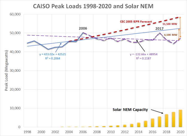
This premise overlooks that these customer resources have met at least a quarter on the energy demand since 2000. The true customer peak is three hours earlier and at least 12,000 megawatts higher than the metered CAISO peak. Based on historic utility costs over that period, annual utility revenue requirements would have increased $14 billion. California already struggled to bring on enough renewable energy over that period—the costs and environmental consequences of using utility generation would likely be even higher.

Claims that customers who save energy cause higher bills for other customers is premised on the unfounded notion that customers are departing from an already existing system built to accommodate their growing future demand. The cost shift analysis starts with today’s situation and then assumes that a customer who installs energy efficiency or rooftop solar is leaving a system already built to serve their current load.

Customers have also added additional loads, including more than one million electric vehicles.  But for the reduction in loads from customer-installed resources, these additional loads would have required billions of dollars of investment in power supply and distribution capacity.  Now, in many cases utilities built the additional capacity anyway – and it is a shortcoming of regulation that these costs were allowed into customer rates when the needed capacity was supplied by customer resources.

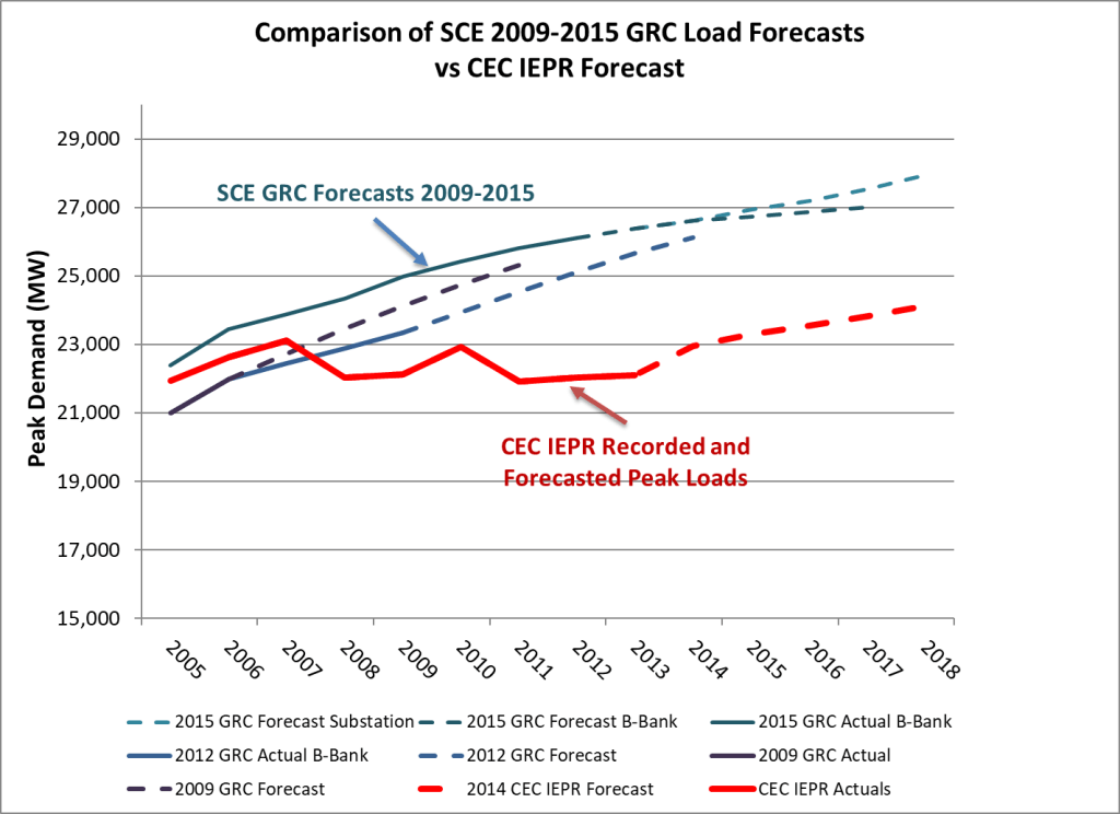
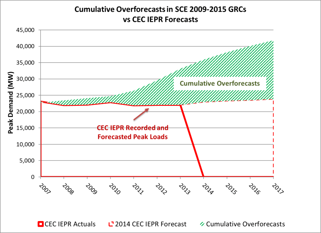
The fact is that a utility system is an aging and dynamic network that is constantly retiring and acquiring equipment to serve an ever-changing group of customers. For California, loads were forecasted to grow another 20% from 2005 to now. Instead, those loads have been flat as consumers have acquired their own resources, including LED lights, insulation, smart thermostats, double paned windows, insulation or solar panels. The metered peak shifted three hours later in the day, but the true customer peak still occurs mid-afternoon but it is met by customer-owned resources instead. A fifth of the true customer peak is now served by rooftop solar and a quarter of the state’s energy load comes from energy efficiency plus DERs. Much of that solar output is captured costlessly in hydro storage and used to meet that later peak.  Any analysis must look at what it would have cost over those two decades to build the resources to serve those loads that instead are now served by individually-invested savings and generation.

We know that generation costs were significantly higher than that today’s costs (thanks to innovation) and that resources located at the point of use saves 30% or more in avoided peak losses and reserve power capacity. We know that those customer resources displaced adding new transmission that costs three times more than the average that is charged in retail rates. We know that the utilities consistently overforecasted the need for distribution infrastructure without consequence, and that the transmission and distribution rate components increased about 300% over the last two decades which is four times faster than inflation. Meanwhile, we also know that utility rates increased at the same pace as utility costs reflected in revenue requirements. This is important because if a other ratepayers were picking up the bills for customers who conserve and self generate, the rates would be increasing faster than revenue requirements as demand decreased. This is the essential element of the “death spiral” concept. There is no evidence of a death spiral yet.

The belief that these “departed” loads could have been served at little additional cost is unfounded based on the empirical evidence. If we conservatively use the average retail generation rate or 8.8 cents per kilowatt-hour in 2023 as representative of the true marginal cost,[4] add 12.5 cents per kilowatt-hour for the marginal cost of transmission, and then add an average of 4.4 cents per kilowatt-hour for avoided distribution costs from the utilities general rate case applications, the base avoided cost is 25.7 cents per kilowatt-hour. We then adjust the generation and transmission costs for 7% line losses and a 15% reserve margin, we are at 30.6 cents per kilowatt-hour for the actual marginal cost at the customer meter. In comparison, the average retail rate was only 27.8 cents per kilowatt in 2023 so customers investing in energy efficiency and rooftop solar are reducing incremental costs by 10%. And of course, this does not include environmental benefits, local economic activity or improved local energy resiliency. The total cost to serve the 89,000 gigawatt-hours saved would be $17 billion or a 30% increase in revenue requirements.

As is often the case, diagnosing the problem doesn’t mean that we have an immediate solution. That said, the objective should be to put utility shareholders at risk for excessive investments made based on optimistic growth forecasts. Having “used and useful” standards for asset utilization rates and unit-of-production depreciation are ways of extending cost recovery that lowers rates. However, those types of solutions are likely to move utilities back to opposing EE programs. The best solution is to create a competitive EE utility like the NW Energy Efficiency Alliance.

Today, we see that California is still struggling to bring on enough clean energy resources to meet its ambitious climate change mitigation goals. Diablo Canyon’s retirement was delayed and the state is not even approaching the threshold for installing renewables to meet the SB 100 clean energy target of 100% by 2045. The only viable alternatives are greater reliance on aggressive energy efficiency paired with electrification and customer-owned renewable generation. Misinterpreting the intention of decoupling should not be used as a barrier to reaching our goals.


[1] California first instituted decoupling in 1978 and then paused it in 1996 for restructuring. The system was restarted in 2002.

[2] It literally takes killing customers to put a utility at financial risk. See “ SDG&E Customers Should Not Pay for 2007 Wildfires: SCOTUS,” NBC 7 News, https://www.nbcsandiego.com/news/local/us-supreme-court-sdge-wildfires-costs-lines-utility-fire-damage/1966157/, October 8, 2019; “PG&E receives maximum sentence for 2010 San Bruno explosion,” ABC 7 News, https://abc7news.com/post/pg-e-receives-maximum-sentence-for-2010-san-bruno-explosion/1722674/, January 28. 2017; “Ex-PG&E execs to pay $117M to settle lawsuit over wildfires,” AP News, https://apnews.com/article/wildfires-business-fires-lawsuits-california-450c961a4c6b467fcfb5465e7b9c5ae7, September 29, 2022; “PG&E Pleads Guilty On 2018 California Camp Fire: ‘Our Equipment Started That Fire’,” NPR CapRadio, https://www.npr.org/2020/06/16/879008760/pg-e-pleads-guilty-on-2018-california-camp-fire-our-equipment-started-that-fire, June 16, 2020. SCE may be facing a similar risk after the Easton Fire in January 2025. “Southern California Edison likely to incur ‘material losses’ related to Eaton fire, executive says,” LA Times, https://www.latimes.com/business/story/2025-04-30/edison-earnings-eaton-fire-losses, April 30, 2025.

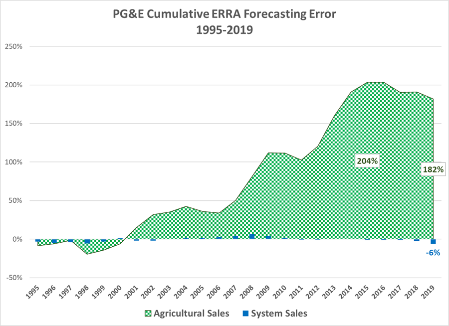
[3] Decoupling delinked profits from actual sales and instead linked them to forecasted sales used to justify infrastructure investment. This removed the risk of overforecasting sales and perhaps falling short on recovering costs. And we see evidence of that practice in both PG&E’s and SCE’s forecasts used to justify investments from 2009 to 2018. The regulatory failure is that the CPUC didn’t go back and audit whether the investments were justified given that the sales didn’t materialize. Decoupling only works with a regulatory scheme that gives strong incentives for cost control.

[4] The 2024 rates were much higher for the utilities but it’s more difficult to calculate the average.

The Jolt: California’s solar blame-game (a podcast interview)

In Wednesday’s episode of The Jolt, Sam looks into why California’s rooftop solar rollout is at risk of stalling.

  • Richard McCann, an expert on California’s energy system and founding partner of the M.Cubed consultancy, joins The Jolt to explain where the state’s officials are making mistakes and what needs to be done to fix them.
  • To reach its 2045 carbon neutrality goal, California needs to build a lot of renewable energy. Rooftop solar has reached about 16 gigawatts of capacity in the state and is a major part of the power mix.
  • But new policy changes, designed to bring down power prices, could derail the rooftop sector’s impressive progress and stunt future growth.

How California got such high rates: the history of missed utility forecasts

A key driver in rising California electricity rates has been distribution costs as shown in the chart above. The distribution rate component has been increasing in lock step with utilities’ revenue requirements since at least 2002. Purported load departure has had no measurable impact on rates as the value of energy efficiency and distributed energy resources have closely mirrored the displaced utility spending over that period.

The most likely source of the increase in distribution costs is overforecasting load growth in the utilities’ General Rate Cases (GRC) after 2006. As described in this California Solar & Storage Association (CalSSA) whitepaper, customer investment in rooftop solar displaced load growth and CAISO peak demands have remained flat, but utility forecasts failed to account for this.

While testifying on behalf of the Agricultural Energy Consumers Association (AECA) in PG&E and SCE GRC Phase IIs from 2009 to 2018 we presented data comparing the accuracy of the utilities forecasts to those from the California Energy Commission’s Integrated Energy Policy Report (IEPR). The IEPR forecasts were consistently much more accurate (and still biased high.) (We moved on to different issues after 2018.)

The first chart shows how PG&E consistently misforecasted. SCE shows the same biased errors in the second chart. An important source of this error appears to be the utilities failing to reconcile the sum of local planning area and division forecasts with the overall system forecast. We asked for data showing this reconciliation but never received evidence of this critical task. Starting in 2018, however, the utilities started using local area forecasts created by the CEC which mitigates this source of error.

Nevertheless, the utilities requested, and the CPUC authorized, large investments that increased the distribution rate base which then rolls into the revenue requirements and rates. The assets installed in excess of demand simply accumulated in the investment ratebase and the additional excess from the next GRC was layered on top. The two charts below show for PG&E and SCE the cumulative amount of overforecast over three GRCs. These imply that each utility was authorized to build substantially more infrastructure than what was actually needed. For PG&E this amounted to 99% by 2019 and for SCE, 76% more by 2017.

These investments facilitated by the forecast errors kept accreting but the CPUC never went back to audit whether theses assets were actually used and useful. If not used and useful, the CPUC could act to disallow recovery of these costs until load growth is sufficient to create a need for these lines and transformers.

In PG&E’s 1996 GRC, AECA showed that the utility was planning to add substantial distribution infrastructure in the farmlands around Fresno for suburban growth that was unlikely to materialize. The CPUC agreed with us and refused to authorize that investment. It took substantial effort by this intervenor to prepare that analysis, but it demonstrated the effectiveness of such oversight that has not been duplicated by the CPUC elsewhere.

This lack of oversight and action is one reason why the policy of decoupling, which separates cost recovery from sales, has failed to control costs in California. Decoupling may have reduced utilities’ opposition to energy efficiency (although now they are coming after rooftop solar which has an identical effect as energy efficiency), but the utilities quickly discovered that the CPUC did not have either the capabilities or the appetite to penalize overinvestment. This is the root cause of California’s high rates.

White paper on how rooftop solar is really a benefit to all ratepayers

In cooperation with the California Solar & Storage Association, M.Cubed is releasing a white paper Rooftop Solar Reduces Costs for All Ratepayers.

As California policy makers seek to address energy affordability in 2025, this report shows why rooftop solar can and has helped control rate escalation. This research stands in direct contrast to claims that rooftop solar is to blame for rising rates. The report shows that the real reason electricity rates have increased dramatically in recent years is out-of-control utility spending and utility profit making, enabled by a lack of proper oversight by regulators.

This work builds on the original short report issued in November 2024, and subsequent replies to critiques by the Public Advocates Office and Professor Severin Borenstein. The supporting workpapers can be found here.

Policy makers wanting to address California’s affordability crisis should reject the utility’s so-called “solar cost shift” and instead partner with consumers who have helped save all ratepayers $1.5 billion in 2024 alone by investing in rooftop solar. The state should prioritize these resources that simultaneously reduce carbon, increase resiliency, and minimize grid spending. This realignment of energy priorities away from what works for investor-owned utilities – spending more on the grid – and toward what works for consumers – spending less – is particularly important in the face of increased electricity consumption due to electrification. More rooftop solar is needed, not less, to control costs for all ratepayers and meet the state’s clean energy goals.

Utilities have peddled a false “cost shift” theory that is based on the concept of “departing load.” Utilities claim that the majority of their costs are fixed. When a customer generates their own power from onsite solar panels, the utilities claim this forces all other ratepayers to pick up a larger share of their “fixed” costs. A close look at hard data behind this theory, however, shows a different picture.

While California’s gross consumption – the “plug load” that is actual electricity consumption – has grown, that growth has been offset by customer-sited rooftop solar. This has kept the state’s peak consumption from the grid remarkably flat over the past twenty years, despite population growth, temperature increases, increased economic activity, and the rise in computers and other electronics in homes and businesses. Rooftop solar has not caused departing load in California. It has avoided load growth. By keeping our electric load on the grid flat, rooftop solar has avoided expensive grid expansion projects, in addition to reducing generation expenses, lowering costs for everyone.

Contrary to messaging from utilities and their regulators, California electricity consumption still peaks in mid-afternoon on hot summer days. There has been so much focus on the evening “net peak,” depicted by the “duck curve,” that many people have lost sight of the true peak. The annual peak in plug load happens when the sun is shining brightest. Clear, hot days lead to both high electricity usage from air conditioning and peak solar output.

The “net peak” is grid-based consumption minus generation from utility-scale solar and wind farms. It is an important dynamic to look at as we seek to reduce non-renewable sources of energy, and it shows us that energy storage will be essential going forward. However, an exclusive focus on net peak misses a bigger picture, particularly when looking at previously installed resources, and hides the value of solar energy.
California’s two million rooftop solar systems installed under net metering, including those that do not have batteries, continue to reduce statewide costs year after year by reducing the true peak. While most new solar systems now have batteries to address the evening net peak, historic solar continues to play a critical role in addressing the mid-day true peak.

Utilities and their regulators ignore these facts and focus the blame of rising rates on consumers seeking relief via rooftop solar. Politicians looking to address a growing crisis of energy affordability in California should reject the scapegoating of working- and middle-class families who have invested their own money in rooftop solar, and should instead promote the continued growth of this important distributed resource to meet growing needs for electricity.

The state is at a crossroads. As we power more of our cars, appliances, and heating with electricity, usage will increase dramatically. Relying entirely on utilities to deliver that energy from faraway power plants on long-distance power lines would involve massive delays and cause costs to rise even higher. Aggressive rooftop solar deployment could offset significant portions of the projected demand increase from electrification, helping control costs in the future.

The real reason for rate increases is runaway utility spending, driven by the utilities’ interest in increasing profits. Utility spending on grid infrastructure at the transmission and distribution levels has increased 130%-260% for each of the utilities over the past 8-12 years. These increases in spending track at a nearly 1:1 ratio with rate increases. This demonstrates that rates have gone up because utility spending has gone up. If utility costs were anything close to fixed and rates kept going up, there could be room for a cost shift argument. Or, if utility spending increased and rates increased significantly more, there could be a cost shift. The data shows neither of these trends. Rates have been increasing commensurate with spending, demonstrating that it is utility spending increases that have caused rates to increase, not consumers investing in clean energy.

Inspired by this faulty approach to measuring solar costs and benefits, the CPUC rolled out a transition from net metering to net billing that was abrupt and extreme. It has caused massive layoffs of skilled solar professionals and bankruptcies or closures of long-standing solar businesses. The poorly managed policy change set the market back ten years. A year and a half after the transition, the market still has not recovered.
California needs more rooftop solar and customer-sited batteries to contain costs and thereby rein in rate increases for all California ratepayers. To get the state back on track, policy makers need to stop attacking solar and adopt smart policies without delay.

• Respect the investments of customers who installed solar under NEM-1 and NEM-2. Do not change the terms of those contracts.
• Reject solar-specific taxes or fees in all forms, via the CPUC, the state budget, or local property taxes.
• Cut red tape in permitting and interconnection, and restore the right of solar contractors to install batteries. Do not use contractor licensing rules at the CSLB to restrict solar contractors from installing batteries.
• Establish a Million Solar Batteries initiative that includes virtual power plants and targeted incentives.
• Fix perverse utility profit motives that drive utilities to spend ratepayer money inefficiently, and even unnecessarily, and that motivate them to fight rooftop solar and other alternative ways to power California families and businesses.
• Launch a new investigation into utility oversight and overhaul the regulatory structure such that government regulators have the ability to properly scrutinize and contain utility spending.

California should be proud of its globally significant rooftop solar market. This solar development has diversified resources, served as a check on runaway utility spending, and helped clean the air all while tapping into private investments in clean energy. As the state looks to decarbonize its economy, the need to generate energy while minimizing capital intensive investments in grid infrastructure makes distributed solar and storage an even higher priority. State regulators need to stop being weak in utility oversight and exercise bold leadership for affordable clean energy that will benefit all ratepayers. California can start by getting back to promoting, not attacking, rooftop solar and batteries for all consumers.

How California’s Rooftop Solar Customers Benefit Other Ratepayers Financially to the Tune of $1.5 Billion

The California Public Utilities Commission’s (CPUC) Public Advocates Office (PAO) issued in August 2024 an analysis that purported to show current rooftop solar customers are causing a “cost shift” onto non-solar customers amounting to $8.5 billion in 2024. Unfortunately, this rather simplistic analysis started from an incorrect base and left out significant contributions, many of which are unique to rooftop solar, made to the utilities’ systems and benefitting all ratepayers. After incorporating this more accurate accounting of benefits, the data (presented in the chart above) shows that rooftop solar customers will in fact save other ratepayers approximately $1.5 billion in 2024.

The following steps were made to adjust the original analysis presented by the PAO:

  1. Rates & Solar Output: The PAO miscalculates rates and overestimates solar output. Retail rates were calculated based on utilities’ advice letters and proceeding workpapers. They incorporate time-of-use rates according to the hours when an average solar customer is actually using and exporting electricity.  The averages are adjusted to include the share of net energy metering (NEM 1.0 and 2.0) and net billing tariff (NBT or “NEM 3.0”) customers (8% to 18% depending on the utility) who are receiving the California Alternate Rates for Energy program’s (CARE) low-income rate discount. (PAO assumed that all customers were non-CARE). In addition, the average solar panel capacity factor was reduced to 17.5% based on the state’s distributed solar database.[1] Accurately accounting for rates and solar outputs amounts to a $2.457 billion in benefits ignored by the PAO analysis.
  2. Self Generation: The PAO analysis included solar self-consumption as being obligated to pay full retail rates. Customers are not obligated to pay for energy to the utility for self generation. Solar output that is self-consumed by the solar customer was removed from the calculation. Inappropriately including self consumption as “lost” revenue in PAO analysis amounts to $3.989 billion in a phantom cost shift that should be set aside.
  3. Historic Utility Savings: The PAO fails to account for the full and accurate amount of savings and the shift in the system created by rooftop solar that has lowered costs and rates. The historic savings are based on distributed solar displacing 15,000 megawatts of peak load and 23,000 gigawatt-hours of energy since 2006 compared to the California Energy Commission’s (CEC) 2005 Integrated Energy Policy Report forecast.[2] Deferred generation capacity valuation starts with the CEC’s cost of a combustion turbine[3] and is trended to the marginal costs filed in the most recent decided general rate cases. Generation energy is the mix of average California Independent System Operator (CAISO) market prices in 2023,[4] and utilities’ average renewable energy contract prices.[5] Avoided transmission costs are conservatively set at the current unbundled retail transmission rate components. Distribution investment savings are the weighted average of the marginal costs included in the utilities’ general case filings from 2007 to 2021. Accounting for utility savings from distributed solar amounts to $2.165 billion ignored by the PAO’s calculation.
  4. Displaced CARE Subsidy: The PAO analysis does not account for savings from solar customers who would otherwise receive CARE subsidies. When CARE customers buy less energy from the utilities, it reduces the total cost of the CARE subsidy born by other ratepayers. This is equally true for energy efficiency. The savings to all non-CARE customers from displacing electricity consumption by CARE customers with self generation is calculated from the rate discount times that self generation. Accounting for reduced CARE subsidies amounts to $157 million in benefits ignored by the PAO analysis.
  5. Customer Bill Payments: The PAO analysis does not account for payments towards fixed costs made by solar customers. Most NEM customers do not offset all of their electricity usage with solar.[6] NEM customers pay an average of $80 to $160 per month, depending on the utility, after installing solar.[7] Their monthly bill payments more than cover what are purported fixed costs, such as the service transformer. A justification for the $24 per month customer charge was a purported under collection from rooftop solar customers.[8] Subtracting the variable costs represented by the Avoided Cost Calculator from these monthly payments, the remainder is the contribution to utility fixed costs, amounting to an average of $70 per month. (In comparison for example, PG&E proposed an average fixed charge of $51 per month in the income graduated fixed charge proceeding.[9]) There is no data available on average NBT bills, but NBT customers also pay at least $15 per month in a minimum fixed charge today.[10] Accounting for fixed cost payments adds $1.18 billion in benefits ignored by the PAO analysis.

The correct analytic steps are as follows:

NEM Net Benefits = [(kWh Generation [Corrected] – kWh Self Use) x Average Retail Rate Compensation [Corrected] )]
– [(kWh Generation [Corrected] – kWh Self Use) x Historic Utility Savings ($/kWh)]
– [CARE/FERA kWh Self Use x CARE/FERA Rate Discount ($/kWh)]
– [(kWh Delivered x (Average Retail Rate ($/kWh) – Historic Utility Savings $(kWh))]

NBT Net Benefits = [(kWh Generation [Corrected] – kWh Self Use) x Average Retail Rate Compensation [Corrected])]
– [(kWh Generation [Corrected] – kWh Self Use) x Avoided Cost (Corrected) ($/kWh)]
– [CARE/FERA kWh Self Use x CARE/FERA Rate Discount ($/kWh)]
– [(Net kWh Delivered x (Average Retail Rate ($/kWh) – Historic Utility Savings $(kWh))]

This analysis is not a value of solar nor a full benefit-cost analysis. It is only an adjusted ratepayer-impact test calculation that reflects the appropriate perspective given the PAO’s recent published analysis. A full benefit-cost analysis would include a broader assessment of impacts on the long-term resource plan, environmental impacts such as greenhouse gas and criteria air pollutant emissions, changes in reliability and resilience, distribution effects including from shifts in environmental impacts, changes in economic activity, and acceleration in technological innovation. Policy makers may also want to consider other non-energy benefits as well such local job creation and supporting minority owned businesses.

This analysis applies equally to one conducted by Severin Borenstein at the University of California’s Energy Institute at Haas. Borenstein arrived at an average retail rate similar to the one used in this analysis, but he also included an obligation for self generation to pay the retail rate, ignored historic utility cost savings and did not include existing bill contributions to fixed costs.

The supporting workpapers are posted here.

Thanks to Tom Beach at Crossborder Energy for a more rigorous calculation of average retail rates paid by rooftop solar customers.


[1] PAO assumed a solar panel capacity factor of 20%, which inflates the amount of electricity that comes from solar. For a more accurate calculation see California Distributed Generation Statistics, https://www.californiadgstats.ca.gov/charts/.

[2] This estimate is conservative because it does not include the accumulated time value of money created by investment begun 18 years ago. It also ignores the savings in reduced line losses (up to 20% during peak hours), avoided reserve margins of at least 15%, and suppressed CAISO market prices from a 13% reduction in energy sales.

[3] CEC, Comparative Costs of California Central Station Electricity Generation Technologies, CEC-200-2007-011-SF, December 2007.

[4] CAISO, 2023 Annual Report on Market Issues & Performance, Department of Market Monitoring, July 29, 2024.

[5] CPUC, “2023 Padilla Report: Costs and Cost Savings for the RPS Program,” May 2023.

[6] Those customers who offset all of their usage pay minimum bills of at least $12 per month.

[7] PG&E, SCE and SDG&E data responses to CALSSA in CPUC Proceeding R.20-08-020, escalated from 2020 to 2024 average rates.

[8] CPUC Decision 24-05-028.

[9] CPUC Proceeding Rulemaking 22-07-005.

[10] The average bill for NBT customer is not known at this time.

“Fixed costs” do not mean “fixed charges”

The California Public Utilities Commission has issued a proposed decision that calls for a monthly fixed charge of $24 for most customers. There is no basis in economic principles that calls for collecting “fixed costs” (too often misidentified) in a fixed charge. This so-called principle gets confused with the second-best solution for regulated monopoly pricing where the monopoly has declining marginal costs that are below average costs which has a two part tariff of a lump sum payment and variable prices at marginal costs. (And Ramsey pricing, which California uses a derivative of that in equal percent marginal cost (EPMC) allocation, also is a second-best efficient pricing method that relies solely on volumetric units.) The evidence for a natural monopoly is that average costs are falling over time as sales expand.

However, as shown by the chart above for PG&E’s distribution and transmission (and SCE’s looks similar), average costs as represented in retail rates are rising. This means that marginal costs must be above average costs. (If this isn’t true then a fully detailed explanation is required—none has been presented so far.) The conditions for regulated monopoly pricing with a lump sum or fixed charge component do not exist in California.

Using the logic that fixed costs should be collected through fixed charges, then the marketplace would be rife with all sorts of entry, access and connection fees at grocery stores, nail salons and other retail outlets as well as restaurants, car dealers, etc. to cover the costs of ownership and leases, operational overhead and other invariant costs. Simply put that’s not the case. All of those producers and providers price on a per unit basis because that’s how a competitive market works. In those markets, customers have the ability to choose and move among sellers, so the seller is forced to recover costs on a single unit price. You might respond, well, cell providers have monthly fixed charges. But that’s not true—those are monthly connection fees that represent the marginal cost of interconnecting to a network. And customers have the option of switching (and many do) to a provider with a lower monthly fee. The unit of consumption is interconnection, which is a longer period than the single momentary instance that economists love because they can use calculus to derive it.

Utility regulation is supposed to mimic the outcome of competitive markets, including pricing patterns. That means that fixed cost recovery through a fixed charge must be limited to a customer-dedicated facility which cannot be used by another customer. That would be the service connection, which has a monthly investment recovery cost of about $10 to $15/month. Everything else must be priced on a volumetric basis as would be in a competitive market. (And the rise of DERs is now introducing true competition into this marketplace.)

The problem is that we’re missing the other key aspect of competitive markets—that investors risk losing their investments due to poor management decisions. Virtually all of the excess stranded costs for California IOUs are due poor management, not “state mandates.” You can look at the differences between in-state IOU and muni rates to see the evidence. (And that an IOU has been convicted of killing nearly 100 people due to malfeasance further supports that conclusion.)

There are alternative solutions to California’s current dilemma but utility shareholders must accept their portion of the financial burden. Right now they are shielded completely as evidenced by record profits and rising share prices.

Retail electricity rate reform will not solve California’s problems

Meredith Fowlie wrote this blog on the proposal to drastically increase California utilities’ residential fixed charges at the Energy Institute at Haas blog. I posted this comment (with some additions and edits) in response.

First, infrastructure costs are responsive to changes in both demand and added generation. It’s just that those costs won’t change for a customer tomorrow–it will take a decade. Given how fast transmission retail rates have risen and have none of the added fixed costs listed here, the marginal cost must be substantially above the current average retail rates of 4 to 8 cents/kWh.

Further, if a customer is being charged a fixed cost for capacity that is being shared with other customers, e.g., distribution and transmission wires, they should be able to sell that capacity to other customers on a periodic basis. While many economists love auctions, the mechanism with the lowest ancillary transaction costs is a dealer market akin a grocery store which buys stocks of goods and then resells. (The New York Stock Exchange is a type of dealer market.) The most likely unit of sale would be in cents per kWh which is the same as today. In this case, the utility would be the dealer, just as today. So we are already in the same situation.

Airlines are another equally capital intensive industry. Yet no one pays a significant fixed charge (there are some membership clubs) and then just a small incremental charge for fuel and cocktails. Fares are based on a representative long run marginal cost of acquiring and maintaining the fleet. Airlines maintain a network just as utilities. Economies of scale matter in building an airline. The only difference is that utilities are able to monopolistically capture their customers and then appeal to state-sponsored regulators to impose prices.

Why are California’s utility rates 30 to 50% or more above the current direct costs of serving customers? The IOUs, and PG&E in particular, over procured renewables in the 2010-2012 period at exorbitant prices (averaging $120/MWH) in part in an attempt to block entry of CCAs. That squandered the opportunity to gain the economics benefits from learning by doing that led to the rapid decline in solar and wind prices over the next decade. In addition, PG&E refused to sell a part of its renewable PPAs to the new CCAs as they started up in the 2014-2017 period. On top of that, PG&E ratepayers paid an additional 50% on an already expensive Diablo Canyon due to the terms of the 1996 Settlement Agreement. (I made the calculations during that case for a client.) And on the T&D side, I pointed out beginning in 2010 that the utilities were overforecasting load growth and their recorded data showed stagnant loads. The peak load from 2006 was the record until 2022 and energy loads have remained largely constant, even declining over the period. The utilities finally started listening the last couple of years but all of that unneeded capital is baked into rates. All of these factors point not to the state or even the CPUC (except as an inept monitor) as being at fault, but rather to the utilities’ mismanagement.

Using Southern California Edison’s (SCE) own numbers, we can illustrate the point. SCE’s total bundled marginal costs in its rate filing are 10.50 cents per kWh for the system and 13.64 cents per kWh for residential customers. In comparison, SCE’s average system rate is 17.62 cents per kWh or 68% higher than the bundled marginal cost, and the average residential rate of 22.44 cents per kWh is 65% higher. From SCE’s workpapers, these cost increases come primarily from four sources.

  1. First, about 10% goes towards various public purpose programs that fund a variety of state-initiated policies such as energy efficiency and research. Much of this should be largely funded out of the state’s General Fund as income distribution through the CARE rate instead. And remember that low income customers are already receiving a 35% discount on rates.
  2. Next, another 10% comes roughly from costs created two decades ago in the wake of the restructuring debacle. The state has now decreed that this revenue stream will instead be used to pay for the damages that utilities have caused with wildfires. Importantly, note that wildfire costs of any kind have not actually reached rates yet. In addition, there are several solutions much less costly than the undergrounding proposed by PG&E and SDG&E, including remote rural microgrids.
  3. Approximately 15% is from higher distribution costs, some of which have been created by over-forecasting load growth over the last 15 years; loads have remained stagnant since 2006.
  4. And finally, around 33% is excessive generation costs caused by paying too much for purchased power agreements signed a decade ago.

An issue raised as rooftop solar spreads farther is the claim that rooftop solar customers are not paying their fair share and instead are imposing costs on other customers, who on average have lower incomes than those with rooftop solar. Yet the math behind the true rate burden for other customers is quite straightforward—if 10% of the customers are paying essentially zero (which they are actually not), the costs for the remaining 90% of the customers cannot go up more than 11% [100%/(100%-10%) = 11% ]. If low-income customers pay only 70% of this—the 11%– then their bills might go up about 8%–hardly a “substantial burden.” (70% x 11% = 7.7%)

As for aligning incentives for electrification, we proposed a more direct alternative on behalf of the Local Government Sustainable Energy Coalition where those who replace a gas appliance or furnace with an electric receive an allowance (much like the all-electric baseline) priced at marginal cost while the remainder is priced at the higher fully-loaded rate. That would reduce the incentive to exit the grid when electrifying while still rewarding those who made past energy efficiency and load reduction investments.

The solution to high rates cannot come from simple rate design; as Old Surfer Dude points out, wealthy customers are just going to exit the grid and self provide. Rate design is just rearranging the deck chairs. The CPUC tried the same thing in the late 1990s with telcom on the assumption that customers would stay put. Instead customers migrated to cell phones and dropped their land lines. The real solution is going to require some good old fashion capitalism with shareholders and associated stakeholders absorbing the costs of their mistakes and greed.

Are PG&E’s customers about to walk?

In the 1990s, California’s industrial customers threatened to build their own self-generation plants and leave the utilities entirely. Escalating generation costs due to nuclear plant cost overruns and too-generous qualifying facilities (QF) contracts had driven up rates, and the technology that made QFs possible also allowed large customers to consider self generating. In response California “restructured” its utility sector to introduce competition in the generation segment and to get the utilities out of that part of the business. Unfortunately the initiative failed, in a big way, and we were left with a hybrid system which some blame for rising rates today.

Those rising rates may be introducing another threat to the utilities’ business model, but it may be more existential this time. A previous blog post described how Pacific Gas & Electric’s 2022 Wildfire Mitigation Plan Update combined with the 2023 General Rate Application could lead to a 50% rate increase from 2020 to 2026. For standard rate residential customers, the average rate could by 41.9 cents per kilowatt-hour.

For an average customer that translates to $2,200 per year per kilowatt of peak demand. Using PG&E’s cost of capital, that implies that an independent self-sufficient microgrid costing $15,250 per kilowatt could be funded from avoiding paying PG&E bills.

The National Renewable Energy Laboratory (NREL) study referenced in this blog estimates that a stand alone residential microgrid with 7 kilowatts of solar paired with a 5 kilowatt / 20 kilowatt-hour battery would cost between $35,000 and $40,000. The savings from avoiding PG&E rates could justify spending $75,000 to $105,000 on such a system, so a residential customer could save up to $70,000 by defecting from the grid. Even if NREL has underpriced and undersized this example system, that is a substantial margin.

This time it’s not just a few large customers with choice thermal demands and electricity needs—this would be a large swath of PG&E’s residential customer class. It would be the customers who are most affluent and most able to pay PG&E’s extraordinary costs. If many of these customers view this opportunity to exit favorably, the utility could truly face a death spiral that encourages even more customers to leave. Those who are left behind will demand more relief in some fashion, but those customers who already defected will not be willing to bail out the company.

In this scenario, what is PG&E’s (or Southern California Edison’s and San Diego Gas & Electric’s) exit strategy? Trying to squeeze current NEM customers likely will only accelerate exit, not stifle it. The recent two-day workshop on affordability at the CPUC avoided discussing how utility investors should share in solving this problem, treating their cost streams as inviolable. The more likely solution requires substantial restructuring of PG&E to lower its revenue requirements, including by reducing income to shareholders.

A misguided perspective on California’s rooftop solar policy

Severin Borenstein at the Energy Institute at Haas has taken another shot at solar rooftop net energy metering (NEM). He has been a continual critic of California’s energy decentralization policies such as those on distribution energy resources (DER) and community choice aggregators (CCAs). And his viewpoints have been influential at the California Public Utilities Commission.

I read these two statements in his blog post and come to a very different conclusions:

“(I)ndividuals and businesses make investments in response to those policies, and many come to believe that they have a right to see those policies continue indefinitely.”

Yes, the investor owned utilities and certain large scale renewable firms have come to believe that they have a right to see their subsidies continue indefinitely. California utilities are receiving subsidies amounting to $5 billion a year due to poor generation portfolio management. You can see this in your bill with the PCIA. This dwarfs the purported subsidy from rooftop solar. Why no call for reforming how we recover these costs from ratepayers and force shareholder to carry their burden? (And I’m not even bringing up the other big source of rate increases in excessive transmission and distribution investment.)

Why wasn’t there a similar cry against bailing out PG&E in not one but TWO bankruptcies? Both PG&E and SCE have clearly relied on the belief that they deserve subsidies to continue staying in business. (SCE has ridden along behind PG&E in both cases to gain the spoils.) The focus needs to be on ALL players here if these types of subsidies are to be called out.

“(T)he reactions have largely been about how much subsidy rooftop solar companies in California need in order to stay in business.”

We are monitoring two very different sets of media then. I see much more about the ability of consumers to maintain an ability to gain a modicum of energy independence from large monopolies that compel that those consumers buy their service with no viable escape. I also see a reactions about how this will undermine directly our ability to reduce GHG emissions. This directly conflicts with the CEC’s Title 24 building standards that use rooftop solar to achieve net zero energy and electrification in new homes.

Along with the effort to kill CCAs, the apparent proposed solution is to concentrate all power procurement into the hands of three large utilities who haven’t demonstrated a particularly adroit ability at managing their portfolios. Why should we put all of our eggs into one (or three) baskets?

Borenstein continues to rely on an incorrect construct for cost savings created by rooftop solar that relies on short-run hourly wholesale market prices instead of the long-term costs of constructing new power plants, transmission rates derived from average embedded costs instead of full incremental costs and an assumption that distribution investment is not avoided by DER contrary to the methods used in the utilities’ own rate filings. He also appears to ignore the benefits of co-locating generation and storage locally–a set up that becomes much less financially viable if a customer adds storage but is still connected to the grid.

Yes, there are problems with the current compensation model for NEM customers, but we also need to recognize our commitments to customers who made investments believing they were doing the right thing. We need to acknowledge the savings that they created for all of us and the push they gave to lower technology costs. We need to recognize the full set of values that these customers provide and how the current electric market structure is too broken to properly compensate what we want customers to do next–to add more storage. Yet, the real first step is to start at the source of the problem–out of control utility costs that ratepayers are forced to bear entirely.

A new agricultural electricity use forecast method holds promise for water use management

Agricultural electricity demand is highly sensitive to water availability. Under “normal” conditions, the State Water Project (SWP) and Central Valley Project (CVP), as well as other surface water supplies, are key sources of irrigation water for many California farmers. Under dry conditions, these water sources can be sharply curtailed, even eliminated, at the same time irrigation requirements are heightened. Farmers then must rely more heavily on groundwater, which requires greater energy to pump than surface water, since groundwater must be lifted from deeper depths.

Over extended droughts, like between 2012 to 2016, groundwater levels decline, and must be pumped from ever deeper depths, requiring even more energy to meet crops’ water needs. As a result, even as land is fallowed in response to water scarcity, significantly more energy is required to water remaining crops and livestock. Much less pumping is necessary in years with ample surface water supply, as rivers rise, soils become saturated, and aquifers recharge, raising groundwater levels.

The surface-groundwater dynamic results in significant variations in year-to-year agricultural electricity sales. Yet, PG&E has assigned the agricultural customer class a revenue responsibility based on the assumption that “normal” water conditions will prevail every year, without accounting for how inevitable variations from these circumstances will affect rates and revenues for agricultural and other customers.

This assumption results in an imbalance in revenue collection from the agricultural class that does not correct itself even over long time periods, harming agricultural customers most in drought years, when they can least afford it. Analysis presented presented by M.Cubed on behalf of the Agricultural Energy Consumers Association (AECA) in the 2017 PG&E General Rate Case (GRC) demonstrated that overcollections can be expected to exceed $170 million over two years of typical drought conditions, with the expected overcollection $34 million in a two year period. This collection imbalance also increases rate instability for other customer classes.

Figure-1 compares the difference between forecasted loads for agriculture and system-wide used to set rates in the annual ERRA Forecast proceedings (and in GRC Phase 2 every three years) and the actual recorded sales for 1995 to 2019. Notably, the single largest forecasting error for system-wide load was a sales overestimate of 4.5% in 2000 and a shortfall in 2019 of 3.7%, while agricultural mis-forecasts range from an under-forecast of 39.2% in the midst of an extended drought in 2013 to an over-forecast of 18.2% in one of the wettest years on record in 1998. Load volatility in the agricultural sector is extreme in comparison to other customer classes.

Figure-2 shows the cumulative error caused by inadequate treatment of agricultural load volatility over the last 25 years. An unbiased forecasting approach would reflect a cumulative error of zero over time. The error in PG&E’s system-wide forecast has largely balanced out, even though the utility’s load pattern has shifted from significant growth over the first 10 years to stagnation and even decline. PG&E apparently has been able to adapt its forecasting methods for other classes relatively well over time.

The accumulated error for agricultural sales forecasting tells a different story. Over a quarter century the cumulative error reached 182%, nearly twice the annual sales for the Agricultural class. This cumulative error has consequences for the relative share of revenue collected from agricultural customers compared to other customers, with growers significantly overpaying during the period.

Agricultural load forecasting can be revised to better address how variations in water supply availability drive agricultural load. Most importantly, the final forecast should be constructed from a weighted average of forecasted loads under normal, wet and dry conditions. The forecast of agricultural accounts also must be revamped to include these elements. In addition, the load forecast should include the influence of rates and a publicly available data source on agricultural income such as that provided by the USDA’s Economic Research Service.

The Forecast Model Can Use An Additional Drought Indicator and Forecasted Agricultural Rates to Improve Its Forecast Accuracy

The more direct relationship to determine agricultural class energy needs is between the allocation of surface water via state and federal water projects and the need to pump groundwater when adequate surface water is not available from the SWP and federal CVP. The SWP and CVP are critical to California agriculture because little precipitation falls during the state’s Mediterranean-climate summer and snow-melt runoff must be stored and delivered via aqueducts and canals. Surface water availability, therefore, is the primary determinant of agricultural energy use, while precipitation and related factors, such as drought, are secondary causes in that they are only partially responsible for surface water availability. Other factors such as state and federal fishery protections substantially restrict water availability and project pumping operations greatly limiting surface water deliveries to San Joaquin Valley farms.

We found that the Palmer Drought Stress Index (PDSI) is highly correlated with contract allocations for deliveries through the SWP and CVP, reaching 0.78 for both of them, as shown in Figure AECA-3. (Note that the correlation between the current and lagged PDSI is only 0.34, which indicates that both variables can be included in the regression model.) Of even greater interest and relevance to PG&E’s forecasting approach, the correlation with the previous year’s PDSI and project water deliveries is almost as strong, 0.56 for the SWP and 0.53 for the CVP. This relationship can be seen also in Figure-3, as the PDSI line appears to lead changes in the project water deliveries. This strong relationship with this lagged indicator is not surprising, as both the California Department of Water Resources and U.S. Bureau of Reclamation account for remaining storage and streamflow that is a function of soil moisture and aquifers in the Sierras.

Further, comparing the inverse of water delivery allocations, (i.e., the undelivered contract shares), to the annual agricultural sales, we can see how agricultural load has risen since 1995 as the contract allocations delivered have fallen (i.e., the undelivered amount has risen) as shown in Figure-4. The decline in the contract allocations is only partially related to the amount of precipitation and runoff available. In 2017, which was among the wettest years on record, SWP Contractors only received 85% of their allocations, while the SWP provided 100% every year from 1996 to 1999. The CVP has reached a 100% allocation only once since 2006, while it regularly delivered above 90% prior to 2000. Changes in contract allocations dictated by regulatory actions are clearly a strong driver in the growth of agricultural pumping loads but an ongoing drought appears to be key here. The combination of the forecasted PDSI and the lagged PDSI of the just concluded water year can be used to capture this relationship.

Finally, a “normal” water year rarely occurs, occurring in only 20% of the last 40 years. Over time, the best representation of both surface water availability and the electrical load dependent on it is a weighted average across the probabilities of different water year conditions.

Proposed Revised Agricultural Forecast

We prepared a new agricultural load forecast for 2021 implementing the changes recommended herein. In addition, the forecasted average agricultural rate was added, which was revealed to be statistically valid. The account forecast was developed using most of the same variables as for the sales forecast to reflect similarities in drivers of both sales and accounts.

Figure-5 compares the performance of AECA’s proposed model to PG&E’s model filed in its 2021 General Rate Case. The backcasted values from the AECA model have a correlation coefficient of 0.973 with recorded values,[1] while PG&E’s sales forecast methodology only has a correlation of 0.742.[2] Unlike PG&E’s model almost all of the parameter estimates are statistically valid at the 99% confidence interval, with only summer and fall rainfall being insignificant.[3]

AECA’s accounts forecast model reflects similar performance, with a correlation of 0.976. The backcast and recorded data are compared in Figure-6. For water managers, this chart shows how new groundwater wells are driven by a combination of factors such as water conditions and electricity prices.