Tag Archives: M.Cubed

How California’s Rooftop Solar Customers Benefit Other Ratepayers Financially to the Tune of $1.5 Billion

The California Public Utilities Commission’s (CPUC) Public Advocates Office (PAO) issued in August 2024 an analysis that purported to show current rooftop solar customers are causing a “cost shift” onto non-solar customers amounting to $8.5 billion in 2024. Unfortunately, this rather simplistic analysis started from an incorrect base and left out significant contributions, many of which are unique to rooftop solar, made to the utilities’ systems and benefitting all ratepayers. After incorporating this more accurate accounting of benefits, the data (presented in the chart above) shows that rooftop solar customers will in fact save other ratepayers approximately $1.5 billion in 2024.

The following steps were made to adjust the original analysis presented by the PAO:

  1. Rates & Solar Output: The PAO miscalculates rates and overestimates solar output. Retail rates were calculated based on utilities’ advice letters and proceeding workpapers. They incorporate time-of-use rates according to the hours when an average solar customer is actually using and exporting electricity.  The averages are adjusted to include the share of net energy metering (NEM 1.0 and 2.0) and net billing tariff (NBT or “NEM 3.0”) customers (8% to 18% depending on the utility) who are receiving the California Alternate Rates for Energy program’s (CARE) low-income rate discount. (PAO assumed that all customers were non-CARE). In addition, the average solar panel capacity factor was reduced to 17.5% based on the state’s distributed solar database.[1] Accurately accounting for rates and solar outputs amounts to a $2.457 billion in benefits ignored by the PAO analysis.
  2. Self Generation: The PAO analysis included solar self-consumption as being obligated to pay full retail rates. Customers are not obligated to pay for energy to the utility for self generation. Solar output that is self-consumed by the solar customer was removed from the calculation. Inappropriately including self consumption as “lost” revenue in PAO analysis amounts to $3.989 billion in a phantom cost shift that should be set aside.
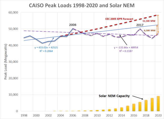
  3. Historic Utility Savings: The PAO fails to account for the full and accurate amount of savings and the shift in the system created by rooftop solar that has lowered costs and rates. The historic savings are based on distributed solar displacing 15,000 megawatts of peak load and 23,000 gigawatt-hours of energy since 2006 compared to the California Energy Commission’s (CEC) 2005 Integrated Energy Policy Report forecast.[2] Deferred generation capacity valuation starts with the CEC’s cost of a combustion turbine[3] and is trended to the marginal costs filed in the most recent decided general rate cases. Generation energy is the mix of average California Independent System Operator (CAISO) market prices in 2023,[4] and utilities’ average renewable energy contract prices.[5] Avoided transmission costs are conservatively set at the current unbundled retail transmission rate components. Distribution investment savings are the weighted average of the marginal costs included in the utilities’ general case filings from 2007 to 2021. Accounting for utility savings from distributed solar amounts to $2.165 billion ignored by the PAO’s calculation.
  4. Displaced CARE Subsidy: The PAO analysis does not account for savings from solar customers who would otherwise receive CARE subsidies. When CARE customers buy less energy from the utilities, it reduces the total cost of the CARE subsidy born by other ratepayers. This is equally true for energy efficiency. The savings to all non-CARE customers from displacing electricity consumption by CARE customers with self generation is calculated from the rate discount times that self generation. Accounting for reduced CARE subsidies amounts to $157 million in benefits ignored by the PAO analysis.
  5. Customer Bill Payments: The PAO analysis does not account for payments towards fixed costs made by solar customers. Most NEM customers do not offset all of their electricity usage with solar.[6] NEM customers pay an average of $80 to $160 per month, depending on the utility, after installing solar.[7] Their monthly bill payments more than cover what are purported fixed costs, such as the service transformer. A justification for the $24 per month customer charge was a purported under collection from rooftop solar customers.[8] Subtracting the variable costs represented by the Avoided Cost Calculator from these monthly payments, the remainder is the contribution to utility fixed costs, amounting to an average of $70 per month. (In comparison for example, PG&E proposed an average fixed charge of $51 per month in the income graduated fixed charge proceeding.[9]) There is no data available on average NBT bills, but NBT customers also pay at least $15 per month in a minimum fixed charge today.[10] Accounting for fixed cost payments adds $1.18 billion in benefits ignored by the PAO analysis.

The correct analytic steps are as follows:

NEM Net Benefits = [(kWh Generation [Corrected] – kWh Self Use) x Average Retail Rate Compensation [Corrected] )]
– [(kWh Generation [Corrected] – kWh Self Use) x Historic Utility Savings ($/kWh)]
– [CARE/FERA kWh Self Use x CARE/FERA Rate Discount ($/kWh)]
– [(kWh Delivered x (Average Retail Rate ($/kWh) – Historic Utility Savings $(kWh))]

NBT Net Benefits = [(kWh Generation [Corrected] – kWh Self Use) x Average Retail Rate Compensation [Corrected])]
– [(kWh Generation [Corrected] – kWh Self Use) x Avoided Cost (Corrected) ($/kWh)]
– [CARE/FERA kWh Self Use x CARE/FERA Rate Discount ($/kWh)]
– [(Net kWh Delivered x (Average Retail Rate ($/kWh) – Historic Utility Savings $(kWh))]

This analysis is not a value of solar nor a full benefit-cost analysis. It is only an adjusted ratepayer-impact test calculation that reflects the appropriate perspective given the PAO’s recent published analysis. A full benefit-cost analysis would include a broader assessment of impacts on the long-term resource plan, environmental impacts such as greenhouse gas and criteria air pollutant emissions, changes in reliability and resilience, distribution effects including from shifts in environmental impacts, changes in economic activity, and acceleration in technological innovation. Policy makers may also want to consider other non-energy benefits as well such local job creation and supporting minority owned businesses.

This analysis applies equally to one conducted by Severin Borenstein at the University of California’s Energy Institute at Haas. Borenstein arrived at an average retail rate similar to the one used in this analysis, but he also included an obligation for self generation to pay the retail rate, ignored historic utility cost savings and did not include existing bill contributions to fixed costs.

The supporting workpapers are posted here.

Thanks to Tom Beach at Crossborder Energy for a more rigorous calculation of average retail rates paid by rooftop solar customers.


[1] PAO assumed a solar panel capacity factor of 20%, which inflates the amount of electricity that comes from solar. For a more accurate calculation see California Distributed Generation Statistics, https://www.californiadgstats.ca.gov/charts/.

[2] This estimate is conservative because it does not include the accumulated time value of money created by investment begun 18 years ago. It also ignores the savings in reduced line losses (up to 20% during peak hours), avoided reserve margins of at least 15%, and suppressed CAISO market prices from a 13% reduction in energy sales.

[3] CEC, Comparative Costs of California Central Station Electricity Generation Technologies, CEC-200-2007-011-SF, December 2007.

[4] CAISO, 2023 Annual Report on Market Issues & Performance, Department of Market Monitoring, July 29, 2024.

[5] CPUC, “2023 Padilla Report: Costs and Cost Savings for the RPS Program,” May 2023.

[6] Those customers who offset all of their usage pay minimum bills of at least $12 per month.

[7] PG&E, SCE and SDG&E data responses to CALSSA in CPUC Proceeding R.20-08-020, escalated from 2020 to 2024 average rates.

[8] CPUC Decision 24-05-028.

[9] CPUC Proceeding Rulemaking 22-07-005.

[10] The average bill for NBT customer is not known at this time.

How to properly calculate the marginal GHG emissions from electric vehicles and electrification

Recently the questions about whether electric vehicles increase greenhouse gas (GHG) emissions and tracking emissions directly to generation on a 24/7 basis have gained saliency. This focus on immediate grid-created emissions illustrates an important concept that is overlooked when looking at marginal emissions from electricity. The decision to consume electricity is more often created by a single large purchase or action, such as buying a refrigerator or a new electric vehicle, than by small decisions such as opening the refrigerator door or driving to the grocery store. Yet, the conventional analysis of marginal electricity costs and emissions assumes that we can arrive at a full accounting of those costs and emissions by summing up the momentary changes in electricity generation measured at the bulk power markets created by opening that door or driving to the store.

But that’s obviously misleading. The real consumption decision that created the marginal costs and emissions is when that item is purchased and connected to the grid. And on the other side, the comparative marginal decision is the addition of a new resource such as a power plant or an energy efficiency investment to serve that new increment of load.

So in that way, your flight to Boston is not whether you actually get on the plane, which is like opening the refrigerator door, but rather your purchase of the ticket which led to the incremental decision by the airline to add another scheduled flight. It’s the share of the fuel use for that added flight which is marginal, just as buying a refrigerator is responsible for the share of the energy from the generator added to serve the incremental long-term load.

There are growing questions about the use of short run market prices as indicators of market value of generation assets for a number of reasons. This paper critiquing “surge” pricing on the grid has one set of aspects that undermine that principle.

Meredith Fowley at the Energy Institute at Haas compared two approaches to measuring the additional GHG emissions from a new electric vehicle. The NREL paper uses the correct approach of looking at longer term incremental resource additions rather than short run operating emissions. The hourly marginal energy use modeled by Holland et al (2022) is not particularly relevant to the question of GHG emissions from added load for several reasons and for that reason any study that doesn’t use a capacity expansion model will deliver erroneous results. In fact, you will get more accurate results from relying on a simple spreadsheet model using capacity expansion than a complex production cost hourly model.

In the electricity grid, added load generally doesn’t just require increased generation from existing plants, but rather it induces investment in new generation (or energy savings elsewhere, which have zero emissions) to meet capacity demands. This is where economists make a mistake thinking that the “marginal” unit is additional generation from existing plants–in a capacity limited system such as the electricity grid, its investment in new capacity.

That average emissions are falling as shown in Holland et al while hourly “marginal” emissions are rising illustrates this error in construction. Mathematically that cannot be happening if the marginal emission metric is correct. The problem is that Holland et al have misinterpreted the value they have calculated. It is in fact not the first derivative of the average emission function, but rather the second partial derivative. That measures the change in marginal emissions, not marginal emissions themselves. (And this is why long-run marginal costs are the relevant costing and pricing metric for electricity, not hourly prices.) Given that 75% of new generation assets in the U.S. were renewables, it’s difficult to see how “marginal” emissions are rising when the majority of new generation is GHG-free.

The second issue is that the “marginal” generation cannot be identified in ceteris paribus (i.e., all else held constant) isolation from all other policy choices. California has a high RPS and 100% clean generation target in the context of beneficial electrification of buildings and transportation. Without the latter, the former wouldn’t be pushed to those levels. The same thing is happening at the federal level. This means that the marginal emissions from building decarbonization and EVs are even lower than for more conventional emission changes.

Further, those consumers who choose beneficial electrification are much more likely to install distributed energy resources that are 100% emission free. Several studies show that 40% of EV owners install rooftop solar as well, far in excess of the state average, (In Australia its 60% of EV owners.) and they most likely install sufficient capacity to meet the full charging load of their EVs. So the system marginal emissions apply only to 60% of EV owners.

There may be a transition from hourly (or operational) to capacity expansion (or building) marginal or incremental emissions, but the transition should be fairly short so long as the system is operating near its reserve margin. (What to do about overbuilt systems is a different conversation.)

There’s deeper problem with the Holland et al papers. The chart that Fowlie pulls from the article showing that marginal emissions are rising above average emissions while average emissions are falling is not mathematically possible. (See for example, https://www.thoughtco.com/relationship-between-average-and-marginal-cost-1147863) For average emissions to be falling, marginal emissions must be falling and below average emissions. The hourly emissions are not “marginal” but more likely are the first derivative of the marginal emissions (i.e., the marginal emissions are falling at a decreasing rate.) If this relationship holds true for emissions, that also means that the same relationship holds for hourly market prices based on power plant hourly costs.

All of that said, it is important to incentivize charging during high renewable hours, but so long as we are adding renewables in a manner that quantitatively matches the added EV load, regardless of timing, we will still see falling average GHG emissions.

It is mathematically impossible for average emissions to fall while marginal emissions are rising if the marginal emission values are ABOVE the average emissions, as is the case in the Holland et al study. What analysts have heuristically called “marginal” emissions, i.e., hourly incremental fuel changes, are in fact, not “marginal”, but rather the first derivative of the marginal emissions. And as you point out the marginal change includes the addition of renewables as well as the change in conventional generation output. Marginal must include the entire mix of incremental resources. How marginal is measured, whether via change in output or over time doesn’t matter. The bottom line is that the term “marginal” must be used in a rigorous economic context, not in a casual manner as has become common.

Often the marginal costs do not fit the theoretical mathematical construct based on the first derivative in a calculus equation that economists point to. In many cases it is a very large discreet increment, and each consumer must be assigned a share of that large increment in a marginal cost analysis. The single most important fact is that for average costs to be rising, marginal costs must be above average costs. Right now in California, average costs for electricity are rising (rapidly) so marginal costs must be above those average costs. The only possible way of getting to those marginal costs is by going beyond just the hourly CAISO price to the incremental capital additions that consumption choices induce. It’s a crazy idea to claim that the first 99 consumers have a tiny marginal cost and then the 100th is assigned the responsibility for an entire new addition such as another flight scheduled or a new distribution upgrade.

We can consider the analogy to unit commitment, and even further to the continuous operation of nuclear power plants. The airline scheduled that flight in part based on the purchase of the plane ticket, not on the final decision just before the gate was closed. Not flying saved a miniscule amount of fuel, but the initial scheduling decision created the bulk of the fuel use for the flight. In a similar manner a power plant that is committed several days before an expected peak load burns fuels while idling in anticipation of that load. If that load doesn’t arrive, that plant avoids a small amount of fuel use, but focusing only on the hourly price or marginal fuel use ignores the fuel burned at a significant cost up to that point. Similarly, Diablo Canyon is run at a constant load year-round, yet there are significant periods–weeks and even months–where Diablo Canyon’s full operational costs are above the CAISO market clearing price average. The nuclear plant is run at full load constantly because it’s dispatch decision was made at the moment of interconnection, not each hour, or even each week or month, which would make economic sense. Renewables have a similar characteristic where they are “scheduled and dispatched” effectively at the time of interconnection. That’s when the marginal cost is incurred, not as “zero-cost” resources each hour.

Focusing solely on the small increment of fuel used as a true measure of “marginal” reflects a larger problem that is distorting economic analysis. No one looks at the marginal cost of petroleum production as the energy cost of pumping one more barrel from an existing well. It’s viewed as the cost of sinking another well in a high cost region, e.g., Kern County or the North Sea. The same needs to be true of air travel and of electricity generation. Adding one more unit isn’t just another inframarginal energy cost–it’s an implied aggregation of many incremental decisions that lead to addition of another unit of capacity. Too often economics is caught up in belief that its like classical physics and the rules of calculus prevail.

A Residential Energy Retrofit Greenhouse Gas Emission Offset Reverse Auction Program

In most local California jurisdictions, the largest share of stationary emissions will continue to come from the existing buildings. On the other hand, achieving zero net energy (ZNE) or zero net carbon (ZNC) for new developments can be cost prohibitive, particularly if incremental transportation emissions are included. A Residential Retrofit Offset Reverse Auction Program (Retrofit Program) aims to balance emission reductions from both new and existing buildings s to lower overall costs, encourage new construction that is more energy efficient, and incentivize a broader energy efficiency marketplace for retrofitting existing buildings.

The program would collect carbon offset mitigation fees from project developers who are unable to achieve a ZNE or ZNC standard with available technologies and measures. The County would then identify eligible low-income residential buildings to be targeted for energy efficiency and electrification retrofits. Contractors then would be invited to bid on how many buildings they could do for a set amount of money.

The approach proposed here is modeled on the Audubon Society’s and The Nature Conservacy’s BirdReturns Program.[1] That program contracts with rice growers in the Sacramento Valley to provide wetlands in the Pacific Flyway. It asks growers to offer a specified amount of acreage with given characteristics for a set price–that’s the “reverse” part of the auction.

A key impediment to further adoption of energy efficiency measures and appliances is that contractors do not have a strong incentive to “upsell” these measures and products to consumers. In general, contractors pass through most of the hardware costs with little markup; their profits are made on the installation and service labor. In addition, contractors are often asked by homeowners and landlords to provide the “cheapest” alternative measured in initial purchase costs without regard to energy savings or long-term expenditures.

The Retrofit Program is intended to change the decision point for contractors to encourage homeowners and landlords to implement upgrades that would create homes and buildings that are more energy efficient. Contractors would bid to install a certain number of measures and appliances that exceed State and local efficiency standards in exchange for payments from the Retrofit Program. The amount of GHG reductions associated with each type of measure and appliance would be predetermined based on a range of building types (e.g., single-family residential by floor-size category, number of floors, and year built). The contractors can use the funds to either provide incentives to consumers or retain those funds for their own internal use, including increased profits. Contractors may choose to provide more information to consumers on the benefits of improved energy efficiency as a means of increasing sales. Contractors would then be compensated from the Offset Program fund upon showing proof that the measures and appliances were installed. The jurisdiction’s building department would confirm the installation of these measures in the normal course of its permit review work.

Funds for the Retrofit Program would be collected as part of an ordinance for new building standards to achieve the no-net increase in GHG emissions. It also could be included as a mitigation measure for projects falling under the purview of the California Environmental Quality Act (CEQA.)

The Retrofit Program would be financed by mitigation payments made by building developers to achieve a no-net increase in GHG emissions. Buildings would be required to meet the lowest achievable GHG emission levels, but then would pay to mitigate any remainders, including for transportation, charged at the current State Cap and Trade Program auction price for an extended collection of annual allowances[2] that cover emissions for the expected life of the building (e.g., 40 years) (CARB 2024).

M.Cubed proposed this financing mechanism for Sonoma County in its climate action plan.


[1] See https://birdreturns.org/

[2] Referred to as a “strip” in the finance industry.

A Working Lands Carbon Mitigation Bank Program

A number of counties in California are largely agricultural, with a few small communities. Most of that agricultural land is intensively farmed, much of it irrigated. This situation presents the opportunity to sequester large amounts of carbon relative to the total greenhouse gas emissions from all county activities. In other words, the county can approach a level of net-zero emissions with a surplus available to share with other jurisdictions, particularly with those in within a county.

Since many of these counties are already planning to use this sequestration strategy to meet its own emission reduction goals, these reductions will be real, additional, and verifiable, meeting the gold standard for use as credits by other jurisdictions. The county has a strong incentive to ensure that these reductions are of sufficient quality to meet its own targets, which should make these attractive to other jurisdictions, unlike other credits offered in the marketplace.

A county would establish a Carbon Mitigation Bank using a similar framework to habitat conservation mitigation banks.[1] The county would establish the parameters that achieve the requisite carbon sequestration and then collect in-lieu fees to cover the costs of the bank’s expenses. By expanding the number of jurisdictions contributing and receiving coverage, overall carbon emissions can be reduced more cost-effectively.

Sequestration from working lands can be achieved at a lower cost than most alternatives. For this reason, a county can use its surplus to finance much of its share of the sequestration program by offering it to cities in the county at a margin above the implementation cost sufficient to cover the county’s share of the costs as well. For example, it may cost $50 per CO2e ton sequestered, and the County may use only half of the potential sequestration to meet its own target. The County could then offer its surplus credits to the other jurisdictions at $100 per ton, which is likely less than the cost of additional reductions elsewhere, to cover the full program costs.

M.Cubed proposed this financing mechanism for both Yolo and Sonoma in their climate action plans. Both counties could potentially sequesters hundreds of thousands of tons annually, implying this could be a major revenue source for meeting broader targets.

Opinion: What’s wrong with basing electricity fees on household incomes

I coauthored this article in the Los Angeles Daily News with Ahmad Faruqui and Andy Van Horn. We critique the proposed income-graduated fixed charge (IGFC) being considered at the California Public Utilities Commission.

Retail electricity rate reform will not solve California’s problems

Meredith Fowlie wrote this blog on the proposal to drastically increase California utilities’ residential fixed charges at the Energy Institute at Haas blog. I posted this comment (with some additions and edits) in response.

First, infrastructure costs are responsive to changes in both demand and added generation. It’s just that those costs won’t change for a customer tomorrow–it will take a decade. Given how fast transmission retail rates have risen and have none of the added fixed costs listed here, the marginal cost must be substantially above the current average retail rates of 4 to 8 cents/kWh.

Further, if a customer is being charged a fixed cost for capacity that is being shared with other customers, e.g., distribution and transmission wires, they should be able to sell that capacity to other customers on a periodic basis. While many economists love auctions, the mechanism with the lowest ancillary transaction costs is a dealer market akin a grocery store which buys stocks of goods and then resells. (The New York Stock Exchange is a type of dealer market.) The most likely unit of sale would be in cents per kWh which is the same as today. In this case, the utility would be the dealer, just as today. So we are already in the same situation.

Airlines are another equally capital intensive industry. Yet no one pays a significant fixed charge (there are some membership clubs) and then just a small incremental charge for fuel and cocktails. Fares are based on a representative long run marginal cost of acquiring and maintaining the fleet. Airlines maintain a network just as utilities. Economies of scale matter in building an airline. The only difference is that utilities are able to monopolistically capture their customers and then appeal to state-sponsored regulators to impose prices.

Why are California’s utility rates 30 to 50% or more above the current direct costs of serving customers? The IOUs, and PG&E in particular, over procured renewables in the 2010-2012 period at exorbitant prices (averaging $120/MWH) in part in an attempt to block entry of CCAs. That squandered the opportunity to gain the economics benefits from learning by doing that led to the rapid decline in solar and wind prices over the next decade. In addition, PG&E refused to sell a part of its renewable PPAs to the new CCAs as they started up in the 2014-2017 period. On top of that, PG&E ratepayers paid an additional 50% on an already expensive Diablo Canyon due to the terms of the 1996 Settlement Agreement. (I made the calculations during that case for a client.) And on the T&D side, I pointed out beginning in 2010 that the utilities were overforecasting load growth and their recorded data showed stagnant loads. The peak load from 2006 was the record until 2022 and energy loads have remained largely constant, even declining over the period. The utilities finally started listening the last couple of years but all of that unneeded capital is baked into rates. All of these factors point not to the state or even the CPUC (except as an inept monitor) as being at fault, but rather to the utilities’ mismanagement.

Using Southern California Edison’s (SCE) own numbers, we can illustrate the point. SCE’s total bundled marginal costs in its rate filing are 10.50 cents per kWh for the system and 13.64 cents per kWh for residential customers. In comparison, SCE’s average system rate is 17.62 cents per kWh or 68% higher than the bundled marginal cost, and the average residential rate of 22.44 cents per kWh is 65% higher. From SCE’s workpapers, these cost increases come primarily from four sources.

  1. First, about 10% goes towards various public purpose programs that fund a variety of state-initiated policies such as energy efficiency and research. Much of this should be largely funded out of the state’s General Fund as income distribution through the CARE rate instead. And remember that low income customers are already receiving a 35% discount on rates.
  2. Next, another 10% comes roughly from costs created two decades ago in the wake of the restructuring debacle. The state has now decreed that this revenue stream will instead be used to pay for the damages that utilities have caused with wildfires. Importantly, note that wildfire costs of any kind have not actually reached rates yet. In addition, there are several solutions much less costly than the undergrounding proposed by PG&E and SDG&E, including remote rural microgrids.
  3. Approximately 15% is from higher distribution costs, some of which have been created by over-forecasting load growth over the last 15 years; loads have remained stagnant since 2006.
  4. And finally, around 33% is excessive generation costs caused by paying too much for purchased power agreements signed a decade ago.

An issue raised as rooftop solar spreads farther is the claim that rooftop solar customers are not paying their fair share and instead are imposing costs on other customers, who on average have lower incomes than those with rooftop solar. Yet the math behind the true rate burden for other customers is quite straightforward—if 10% of the customers are paying essentially zero (which they are actually not), the costs for the remaining 90% of the customers cannot go up more than 11% [100%/(100%-10%) = 11% ]. If low-income customers pay only 70% of this—the 11%– then their bills might go up about 8%–hardly a “substantial burden.” (70% x 11% = 7.7%)

As for aligning incentives for electrification, we proposed a more direct alternative on behalf of the Local Government Sustainable Energy Coalition where those who replace a gas appliance or furnace with an electric receive an allowance (much like the all-electric baseline) priced at marginal cost while the remainder is priced at the higher fully-loaded rate. That would reduce the incentive to exit the grid when electrifying while still rewarding those who made past energy efficiency and load reduction investments.

The solution to high rates cannot come from simple rate design; as Old Surfer Dude points out, wealthy customers are just going to exit the grid and self provide. Rate design is just rearranging the deck chairs. The CPUC tried the same thing in the late 1990s with telcom on the assumption that customers would stay put. Instead customers migrated to cell phones and dropped their land lines. The real solution is going to require some good old fashion capitalism with shareholders and associated stakeholders absorbing the costs of their mistakes and greed.

In the LA Times – looking for alternative solutions to storm outages

I was interviewed by a Los Angeles Times reporter about the recent power outages in Northern California as result of the wave of storms. Our power went out for 48 hours New Year’s Eve and again for 12 hours the next weekend:

After three days without power during this latest storm series, Davis resident Richard McCann said he’s seriously considering implementing his own microgrid so he doesn’t have to rely on PG&E.

“I’ve been thinking about it,” he said. McCann, whose work focuses on power sector analysis, said his home lost power for about 48 hours beginning New Year’s Eve, then lost it again after Saturday for about 12 hours.

While the storms were severe across the state, McCann said Davis did not see unprecedented winds or flooding, adding to his concerns about the grid’s reliability.

He said he would like to see California’s utilities “distributing the system, so people can be more independent.”

“I think that’s probably a better solution rather than trying to build up stronger and stronger walls around a centralized grid,” McCann said.

Several others were quoted in the article offering microgrids as a solution to the ongoing challenge.

Widespread outages occurred in Woodland and Stockton despite winds not being exceptionally strong beyond recent experience. Given the widespread outages two years ago and the three “blue sky” multi hour outages we had in 2022 (and none during the September heat storm when 5,000 Davis customers lost power), I’m doubtful that PG&E is ready for what’s coming with climate change.

PG&E instead is proposing to invest up to $40 billion in the next eight years to protect service reliability for 4% of their customers via undergrounding wires in the foothills which will raise our rates up to 70% by 2030! There’s an alternative cost effective solution that would be 80% to 95% less sitting before the Public Utilities Commission but unlikely to be approved. There’s another opportunity to head off PG&E and send some of that money towards fixing our local grid coming up this summer under a new state law.

While winds have been strong, they have not been at the 99%+ range of experience that should lead to multiple catastrophic outcomes in short order. And having two major events within a week, plus the outage in December 2020 shows that these are not statistically unusual. We experienced similar fierce winds without such extended outages. Prior to 2020, Davis only experienced two extended outages in the previous two decades in 1998 and 2007. Clearly the lack of maintenance on an aging system has caught up with PG&E. PG&E should reimagine its rural undergrounding program to mitigate wildfire risk to use microgrids instead. That will free up most of the billons it plans to spend on less than 4% of its customer base to instead harden its urban grid.

David Mitchell in the LA Times: As drought drives prices higher, millions of Californians struggle to pay for water

M.Cubed Partner David Mitchell was interviewed for an article on rising residential water rates in California in this October 24 article:

Across the state, water utility prices are escalating faster than other “big ticket” items such as college tuition or medical costs, according to David Mitchell, an economist specializing in water.

“Cost containment is going to become an important issue for the sector in the coming years” as climate change worsens drought and water scarcity, he said.

The price of water on the Nasdaq Veles California Water Index, which is used primarily for agriculture, hit $1,028.86 for an acre-foot on Oct. 20 — a roughly 40% increase since the start of the year. An acre-foot of water, or approximately 326,000 gallons, is enough to supply three Southern California households for a year.

Mitchell said there are short- and long-term factors contributing to rising water costs.

Long-term factors include the replacement of aging infrastructure, new treatment standards, and investments in insurance, projects and storage as hedges against drought.

In the short term, however, drought restrictions play a significant role. When water use drops, urban water utilities — which mostly have fixed costs — earn less revenue. They adjust their rates to recover that revenue, either during or after the drought.

“So it’s not right now a pretty picture,” Mitchell said.

David Mitchell’s practice areas include benefit-cost analysis, regional economic impact assessment, utility rate setting and financial planning, and natural resource valuation. Mr. Mitchell has in-depth knowledge of the water supply, water quality and environmental management challenges confronting natural resource management agencies.

The real lessons from California’s 2000-01 electricity crisis and what they mean for today’s markets

The recent reliability crises for the electricity markets in California and Texas ask us to reconsider the supposed lessons from the most significant extended market crisis to date– the 2000-01 California electricity crisis. I wrote a paper two decades ago, The Perfect Mess, that described the circumstances leading up to the event. There have been two other common threads about supposed lessons, but I do not accept either as being true solutions and are instead really about risk sharing once this type of crisis ensues rather than being useful for preventing similar market misfunctions. Instead, the real lesson is that load serving entities (LSEs) must be able to sign long-term agreements that are unaffected and unfettered directly or indirectly by variations in daily and hourly markets so as to eliminate incentives to manipulate those markets.

The first and most popular explanation among many economists is that consumers did not see the swings in the wholesale generation prices in the California Power Exchange (PX) and California Independent System Operator (CAISO) markets. In this rationale, if consumers had seen the large increases in costs, as much as 10-fold over the pre-crisis average, they would have reduced their usage enough to limit the gains from manipulating prices. Consumers should have shouldered the risks in the markets in this view and their cumulative creditworthiness could have ridden out the extended event.

This view is not valid for several reasons. The first and most important is that the compensation to utilities for stranded assets investment was predicated on calculating the difference between a fixed retail rate and the utilities cost of service for transmission and distribution plus the wholesale cost of power in the PX and CAISO markets. Until May 2000, that difference was always positive and the utilities were well on the way to collecting their Competition Transition Charge (CTC) in full before the end of the transition period March 31, 2002. The deal was if the utilities were going to collect their stranded investments, then consumers rates would be protected for that period. The risk of stranded asset recovery was entirely the utilities’ and both the California Public Utilities Commission in its string of decisions and the State Legislature in Assembly Bill 1890 were very clear about this assignment.

The utilities had chosen to support this approach linking asset value to ongoing short term market valuation over an upfront separation payment proposed by Commissioner Jesse Knight. The upfront payment would have enabled linking power cost variations to retail rates at the outset, but the utilities would have to accept the risk of uncertain forecasts about true market values. Instead, the utilities wanted to transfer the valuation risk to ratepayers, and in return ratepayers capped their risk at the current retail rates as of 1996. Retail customers were to be protected from undue wholesale market risk and the utilities took on that responsibility. The utilities walked into this deal willingly and as fully informed as any party.

As the transition period progressed, the utilities transferred their collected CTC revenues to their respective holding companies to be disbursed to shareholders instead of prudently them as reserves until the end of the transition period. When the crisis erupted, the utilities quickly drained what cash they had left and had to go to the credit markets. In fact, if they had retained the CTC cash, they would not have had to go the credit markets until January 2001 based on the accounts that I was tracking at the time and PG&E would not have had a basis for declaring bankruptcy.

The CTC left the market wide open to manipulation and it is unlikely that any simple changes in the PX or CAISO markets could have prevented this. I conducted an analysis for the CPUC in May 2000 as part of its review of Pacific Gas & Electric’s proposed divestiture of its hydro system based on a method developed by Catherine Wolfram in 1997. The finding was that a firm owning as little as 1,500 MW (which included most merchant generators at the time) could profitably gain from price manipulation for at least 2,700 hours in a year. The only market-based solution was for LSEs including the utilities to sign longer-term power purchase agreements (PPAs) for a significant portion (but not 100%) of the generators’ portfolios. (Jim Sweeney briefly alludes to this solution before launching to his preferred linkage of retail rates and generation costs.)

Unfortunately, State Senator Steve Peace introduced a budget trailer bill in June 2000 (as Public Utilities Code Section 355.1, since repealed) that forced the utilities to sign PPAs only through the PX which the utilities viewed as too limited and no PPAs were consummated. The utilities remained fully exposed until the California Department of Water Resources took over procurement in January 2001.

The second problem was a combination of unavailable technology and billing systems. Customers did not yet have smart meters and paper bills could lag as much as two months after initial usage. There was no real way for customers to respond in near real time to high generation market prices (even assuming that they would have been paying attention to such an obscure market). And as we saw in the Texas during Storm Uri in 2021, the only available consumer response for too many was to freeze to death.

This proposed solution is really about shifting risk from utility shareholders to ratepayers, not a realistic market solution. But as discussed above, at the core of the restructuring deal was a sharing of risk between customers and shareholders–a deal that shareholders failed to keep when they transferred all of the cash out of their utility subsidiaries. If ratepayers are going to take on the entire risk (as keeps coming up) then either authorized return should be set at the corporate bond debt rate or the utilities should just be publicly owned.

The second explanation of why the market imploded was that the decentralization created a lack of coordination in providing enough resources. In this view, the CDWR rescue in 2001 righted the ship, but the exodus of the community choice aggregators (CCAs) again threatens system integrity again. The preferred solution for the CPUC is now to reconcentrate power procurement and management with the IOUs, thus killing the remnants of restructuring and markets.

The problem is that the current construct of the PCIA exit fee similarly leaves the market open to potential manipulation. And we’ve seen how virtually unfettered procurement between 2001 and the emergence of the CCAs resulted in substantial excess costs.

The real lessons from the California energy crisis are two fold:

  • Any stranded asset recovery must be done as a single or fixed payment based on the market value of the assets at the moment of market formation. Any other method leaves market participants open to price manipulation. This lesson should be applied in the case of the exit fees paid by CCAs and customers using distributed energy resources. It is the only way to fairly allocate risks between customers and shareholders.
  • LSEs must be able unencumbered in signing longer term PPAs, but they also should be limited ahead of time in the ability to recover stranded costs so that they have significant incentives to prudently procure resources. California’s utilities still lack this incentive.

Close Diablo Canyon? More distributed solar instead

More calls for keeping Diablo Canyon have coming out in the last month, along with a proposal to match the project with a desalination project that would deliver water to somewhere. (And there has been pushback from opponents.) There are better solutions, as I have written about previously. Unfortunately, those who are now raising this issue missed the details and nuances of the debate in 2016 when the decision was made, and they are not well informed about Diablo’s situation.

One important fact is that it is not clear whether continued operation of Diablo is safe. Unit No. 1 has one of the most embrittled containment vessels in the U.S. that is at risk during a sudden shutdown event.

Another is that the decision would require overriding a State Water Resources Control Board decision that required ending the use of once-through cooling with ocean water. That cost was what led to the closure decision, which was 10 cents per kilowatt-hour at current operational levels and in excess of 12 cents in more likely operations.

So what could the state do fairly quickly for 12 cents per kWh instead? Install distributed energy resources focused on commercial and community-scale solar. These projects cost between 6 and 9 cents per kWh and avoid transmission costs of about 4 cents per kWh. They also can be paired with electric vehicles to store electricity and fuel the replacement of gasoline cars. Microgrids can mitigate wildfire risk more cost effectively than undergrounding, so we can save another $40 billion there too. Most importantly they can be built in a matter of months, much more quickly than grid-scale projects.

As for the proposal to build a desalination plant, pairing one with Diablo would both be overkill and a logistical puzzle. The Carlsbad plant produces 56,000 acre-feet annually for San Diego County Water Agency. The Central Coast where Diablo is located has a State Water Project allocation of 45,000 acre-feet which is not even used fully now. That plant uses 35 MW or 1.6% of Diablo’s output. A plant built to use all of Diablo’s output could produce 3.5 million acre-feet, but the State Water Project would need to be significantly modified to move the water either back to the Central Valley or beyond Santa Barbara to Ventura. All of that adds up to a large cost on top of what is already a costly source of water of $2,500 to $2,800 per acre-foot.